PR_QG_A AND PR_QG_B: gravimetric quasi-geoid models for the Paraná state, Brazil, referenced to the IHRS and BVDI

Abstract:

This study aims to compute two gravimetric quasi-geoid models for the Paraná state, Brazil, called PR_QG_A and PR_QG_B. The first referenced to the International Height Reference System and the second to the Brazilian Vertical Local Datum in Imbituba. A dataset of 67,618 terrestrial and oceanic gravimetric data has been used. The Remove-Compute-Restore technique was employed in conjunction with the scalar-free solution of the Geodesy Boundary Value Problem, taking into account the zero and first-order terms of Molodenskii’s series. Before computing the models, an optimal configuration in terms of transition degree/order, modification degree of Stokes’ kernel, and cap size was identified. Iterative multiple pointwise solutions were calculated for GNSS/leveling co-location stations. After validating the quasi-geoid models against GNSS/leveling data, both presented a standard deviation of 0.199 m in terms of height anomaly. For additional validation purposes, the results were compared with those obtained from the SAM_QGEOID2023 model. The differences in terms of standard deviation were approximately 2 mm. However, the values can differ by up to 0.707 meters in certain regions. The computed models will be able to provide normal height values more practically and economically, representing an alternative to leveling, within the indicated accuracy limit.

Keywords:
quasi-geoid model; Paraná - Brazil; International Height Reference System; Brazilian Vertical Local Datum in Imbituba

1. Introduction

One of the ways to obtain normal heights in a more practical and economical way is by using GNSS positioning in conjunction with a quasi-geoid model. It represents an alternative to the leveling procedure within a certain accuracy threshold. This is particularly relevant because, depending on the distance covered, leveling can become costly or impractical. Costs can be substantial, not only in financial terms but also regarding planning, execution, and the processing time of the measured data. Specifically in the Paraná state, there can be dozens of kilometers to cover with leveling, depending on the region. In addition, the High Precision Altimetry Network stations are not always found, and when found, they may not be in a good state of conservation.

Recently, taking into account the adoption of normal heights in Brazil, a model for converting ellipsoidal heights into normal heights was developed and made available by the Brazilian Institute of Geography and Statistics (IBGE), called hgeoHNOR2020 (IBGE 2022). However, it is not a gravimetric quasi-geoid model (GQGM), since conventional methodologies for modeling the gravity field were not used (IBGE 2022). Furthermore, improvements to the MAPGEO2015 geoid model (Blitzkow et al. 2016), on which the model is based, are possible. For example, with the use of more recent gravimetric data, and with the use of more recent and accurate Global Geopotential Models (GGMs), Topographic Gravity Field Models (TGFMs), and Digital Surface Models (DSMs).

In addition, there is currently the implementation of the so-called Global Geodetic Reference System (GGRS), proposed by the United Nations in 2015 (UN 2015), with a view to sustainable development (Resolution A/RES/69/266). It is an integrated System, whose part related to the terrestrial gravity field incorporates the International Height Reference System (IHRS - IAG 2019) and the International Terrestrial Gravity Reference System (ITGRS - IAG 2019). In Brazil, however, the Brazilian Local Vertical Data Imbituba and Santana (BVDI and BVDS) are still in use, while the International Height Reference Frame (IHRF - realization of the IHRS) has not yet been adopted, which should occur in the coming years.

When thinking about such facts specifically for the Paraná state, Brazil, our study aims to compute two GQGMs, one referenced to the IHRS and the other to the BVDI. A more recent and more accurate database currently available has been used in conjunction with an optimal configuration in terms of transition d/o (TDO), modification degree of Stokes’ kernel, and cap size. The use of the GQGMs will allow the conversion of ellipsoidal heights into normal heights already referenced directly to the IHRS or BVDI, in order to provide altimetric information related to the Earth’s gravity field in a more economical, practical, and unified way, in applications where they are necessary.

It is relevant to mention that, although there are previously computed GQGMs for the state, such as SAM_QGEOID2023 (Guimarães et al. 2025), they are not referenced to either the IHRS or the BVDI, and are not made available in mean-tide concept, which is necessary if one wishes to directly obtain vertical coordinates referenced to the IHRS. Furthermore, the models were computed using a different methodology from those used in previous models and additional gravity data in some regions. In addition, it is pertinent to mention that, within the scope of the IHRF, Sánchez et al. (2021) recommends redundant solutions aiming for validations, which could be extended to the computation of GQGMs as well.

2. Gravimetric quasi-geoid models computation

2.1 Study area, dataset and preprocessing

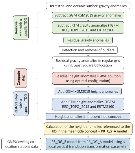
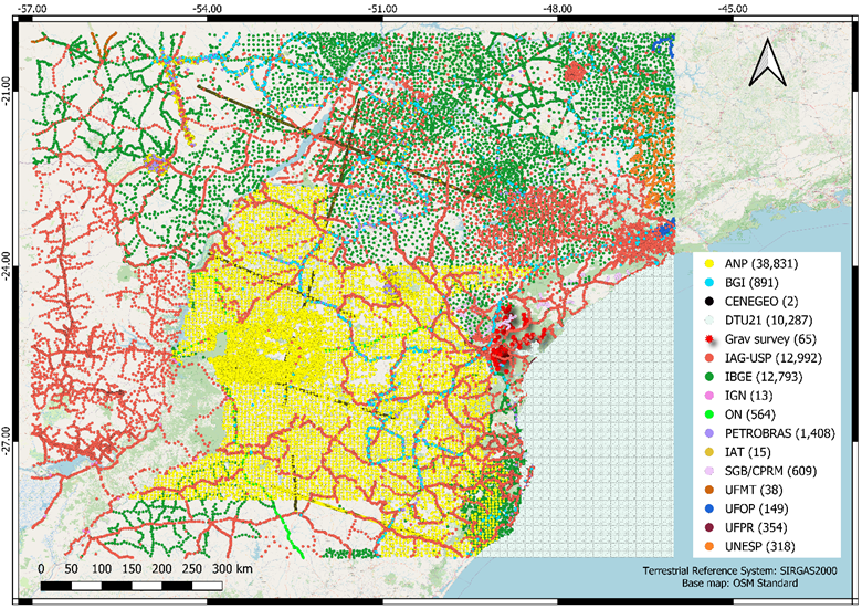
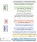
Model computation followed the simplified workflow outlined in Figure 1. Initial procedures consisted of the collection, organization, processing, and analysis of gravimetric data. In the collection step, all continental and oceanic gravimetric data available in the study area were obtained. The study area extends between latitudes 20° S and 29° S and longitudes 46° W and 57° W. The data with their spatial locations, their sources of acquisition, and quantities are presented in Figure 2.

Figure 1:
Simplified workflow followed for the model computation.

Figure 2:
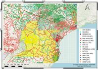
Spatial location of continental and oceanic gravimetric data in the study area, their respective sources and quantities.

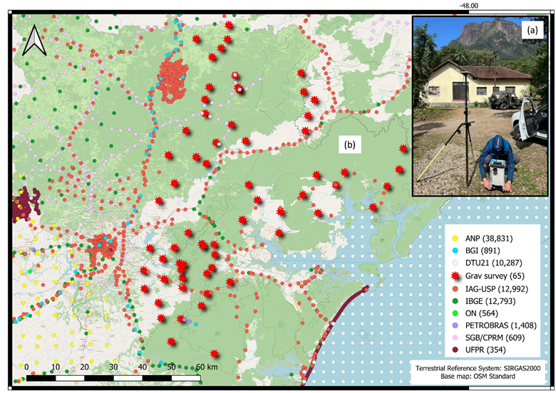
Continental data was obtained from public agencies free of charge, such as the National Petroleum, Natural Gas and Biofuels Agency (ANP); Petróleo Brasileiro S.A. (Petrobras); Brazilian Geological Service (Mineral Resources Research Company - SGB/CPRM); National Observatory (ON); Institute of Astronomy, Geophysics and Atmospheric Sciences of the University of São Paulo (IAG/USP), IBGE, Water and Land Institute of Paraná (IAT - PR), Federal University of Paraná (UFPR), Federal University of Mato Grosso (UFMT), Federal University of Ouro Preto (UFOP), Universidade Estadual Paulista (Unesp), Federal University of Rio Grande do Sul (UFRGS), Bureau Gravimetrique International (BGI), Centro de Estudos de Geodesia (CENEGEO), and National Geographic Institute (IGN) of Argentina. Data obtained from the thesis developed in the graduate programs in Geology and Geodetic Sciences at UFPR were also used. In addition, after identifying some regions without gravity data, a set of 65 data was obtained from a gravimetric survey using a Scintrex CG-5 gravimeter (Figure 3). In total, 104,706 terrestrial data were obtained.

For the oceanic region, a dataset of 10,287 points with gravity anomaly values was obtained from the DTU21GRA model developed by the National Space Institute at the Technical University of Denmark (ANDERSEN et al. 2023). All terrestrial and oceanic gravity data were transformed from mean-tide to zero-tide concept using Eakman (1989) equations, as recommended by Sánchez et al. (2021) in the context of IHRF. The geodetic coordinates were used in the tide-free concept, referenced to the Brazilian Geodetic System (BGS), which is a national densification of the SIRGAS 2000.

Figure 3:
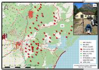
(a) Example of gravity measurements carried out with Scintrex-CG5, and (b) set of 65 data obtained from a gravimetric survey in areas without prior gravimetric data.

In the organization and pre-processing step, duplicate terrestrial data were eliminated. For detection and removal, a routine was built in a MATLAB environment, using threshold values for distance and gravity of 0.003° and 0.5 mGal, respectively. In total, 47,375 duplicated data were found, leaving a total of 57,331 data points for use.

Subsequently, the surface (Molodenskii) gravity anomaly values ($∆g_M$) were calculated in zero-tide concept, taking into account the atmospheric corrections obtained according to the Wenzel (1985) model (Eq. 1). The normal gravity values on the Telluroid were also transformed from the mean-tide to zero-tide concept before calculating the gravity anomalies. In accordance with the established for the IHRS (Wang et al. 2021), the Reference Ellipsoid adopted was the GRS80 (Moritz 2000).

$∆g_M=g-{\gamma }_0\left[1-2\left(1+f+m-2f\phi \right)\frac{H^{*}}{a}+3{\left(\frac{H^{*}}{a}\right)}^2+24{\left(\frac{H^{*}}{a}\right)}^3\right]+\delta g_{ATM}$ (1)

with:

$\delta g_{ATM}=0.874-9.9\times {10}^{-5}{H}^{*}+3.5625\times {10}^{-9}{H^{*}}^2$ (2)

where g is the gravity observation on the terrestrial surface; γ ₀ is the normal gravity on the reference ellipsoid, computed by Gravity Formula 1980 (Moritz 2000); f is the geometrical flattening of the ellipsoid; m is the ratio of centrifugal and gravity acceleration at its equator; φ is the geodetic latitude; a is the equatorial radius; and H* is the approximated normal height obtained from GGM XGM2019e (Zingerle et al. 2020) and TGFM ERTM2160 (Hirt et al. 2014) models in conjunction.

2.2 Model computation

Before computation the GQGMs, pointwise normal height values were calculated for the positions of a set of 97 GNSS/leveling co-location stations from BGS, whose data can be found in the IBGE geodetic database. Using such data as a reference, we identified an optimal configuration in terms of TDO, modification degree of Stokes’ kernel (L), and cap size (ψ ₀ ), as in Foroughi et al. (2017), Claessens and Filmer (2020), and Padilha et al. (2026). The term TDO herein refers to the degree/order (d/o) in which the spectral content modeled by the GGM is limited and the content modeled by the RTM technique begins sequentially. Thus, using the RCR technique, multiple solutions were obtained iteratively, with TDO values of 300, 500, and 760, L values tested from 0 to TDO, with an interval of 30, and ψ ₀ values tested from 0 to 2.5°, every 0.1°.

In the Remove step, the GGM XGM2019 was used as the reference gravity field. For the RTM effect, in spectral domain, the REQ_TOPO_2015 (Grombein et al. 2016) and ERTM2160 (Hirt et al. 2014) models were used together, both developed with the Rock Equivalent Topography (RET) configuration. For the case of the REQ_TOPO_2015 model, the spectral content used was from TDO+1 to 2189 d/o. In the case of the ERTM2160 model, the modeled content was from 2190 to 81000 d/o, which is specific to this model. The residual surface gravity anomaly values were obtained by Eq. (3). It is important to highlight that the missing part of the spectral content (omission errors) and the commission errors were modeled with the GBVP solution.

$∆g_{M_{res}}=∆g_M-∆g_{M_{XGM2019}}-\left(∆g_{M_{RE{Q}_{TOP{O}_{2015}}}}+∆g_{M_{ERTM2160}}\right)$ (3)

where ∆g _{M_XGM2019} corresponds to the contribution of GGM XGM2019 up to TOD, ∆g _{M_REQ_TOPO_2015} corresponds to the contribution of the TGFM REQ_TOPO_2015 from TOD+1 up to 2189 d/o, and ∆g _{M_ERTM2160} corresponds to the contribution of the TGFM ERTM2160 from 2190 to approximately 81000 d/o.

With the smoothed gravity field data, outliers in continental data were identified and removed. These were detected by applying the 3-sigma rule to the sample sets of ten closest neighbors to each point (empirically defined quantity). In total, 61 points were considered outliers.

To obtain the regular grid of residual gravity anomalies, in each TOD configuration, interpolation/adjustment by the Least Squares Collocation Method was used. Several adjusted covariance functions (ACFs) were compared with empirical covariance functions (ECFs) in order to obtain a more precise interpolation/adjustment. The following functions were tested: exponential, Fourier, Gaussian, Hirvonen, 2^nd order Markov, Sine polynomial, Polynomial, and Reilly. For more information on the mathematical model of these functions, see Duquenne et al. (2005). The choice of the most appropriate ACF was based on the analysis of the coefficient of determination (R ² ) value. The resolution of the grids, determined from the average surface density of gravimetric data in the study area, taking into account the Nyquist wavelength, was 3’, which was the resolution adopted for the final grids of the PR_QG_A and PR_QG_B GQGMs.

In the Compute step, the residual height anomaly values for each computation point P (${\zeta }_{{res}_P}$) were obtained from the scalar-free solution of the GBVP, using the zero and first-order terms of Molodenskii’s series (G ₀ and G ₁ ). Thus, we have (Heiskanen and Moritz 1967):

${\zeta }_{{res}_P}={\zeta }_{{0_{res}}_P}+{\zeta }_{{1_{res}}_P}$ (4)

with:

${\zeta }_{{0_{res}}_P}=\frac{R}{4\pi {\gamma }_{P\text{'}}}{\iint }_{\sigma }^{}{G}_0{S}^{WG}\left(\psi \right)d\sigma$ (5)

${\zeta }_{{1_{res}}_P}=\frac{R}{4\pi {\gamma }_{P^{\text{'}}}}{\iint }_{\sigma }^{}{G}_1{S}^{WG}\left(\psi \right)d\sigma$ (6)

in which R is the radius of a sphere with the same volume as the Reference Ellipsoid; ${\gamma }_{P^{\mathrm{\text{'}}}}$ is the normal gravity value in the projection of the computation point P on the Telluroid; σ is the integration area; $G_0=∆g_{M_{res}}$; and G ₁ is given by (Heiskanen and Moritz 1967):

$G_1=\frac{R^2}{2\pi }{\iint }_{\sigma }^{\mathrm{}}\frac{H-H_P}{l_0^3}\left[∆g_{M_{res}}+\frac{3{\gamma }_Q}{2R}{\zeta }_{{0_{res}}_P}\right]d\sigma$ (7)

where H _P and H are the heights of the computation and running integration points, respectively; and l ₀ is the distance between these points. In Eq. (5) and (6), the S ^WG (ψ) term is the spheroidal Stokes function with Wong and Gore (1969)’s modification given by:

$S^{WG}\left(\psi \right)=S\left(\psi \right)-\sum _{n=2}^L\frac{2n+1}{n-1}{P}_n\left(\cos \psi \right)$ (8)

where ψ is the angular distance between the computation point and the running integration points, S(ψ) is the unmodified spheroidal Stokes function, and P _n (cosψ) is the Legendre polynomial of degree n.

The convolution integrals in Equations (5), (6) and (7) were solved through numerical solution, using the Newton-Cotes method, in vector form, in MATLAB environment (MATLAB 2024; Abdalla & Ferreira 2022). The routines were previously developed and validated within the scope of the Colorado 1 cm Geoid Experiment (Padilha et al. 2026), which today serves as the state of the art in accurate high-resolution regional gravity field modeling (Wang et al. 2021).

The Restore step was carried out according to the tested TOD, using the same gravity field models, including the zero-degree terms for reference to the IHRS, according to Eq. (9). Then, the normal height values referenced to the IHRS for each computation point P (${{H^{*}}_{IHRS}}_P$) were obtained according to Eq. (10).

${\zeta }_{{prov}_P}={\zeta }_{{res}_P}+{\zeta }_{{XGM2019}_P}+\left({\zeta }_{{RE{Q}_{TOP{O}_{2015}}}_P}+{\zeta }_{{ERTM2160}_P}\right)+\frac{{GM}_{GGM}-{GM}_{GRS80}}{r_P{\gamma }_{P^{\mathrm{\text{'}}}}}-\frac{{W_0}_{IHRS}-U_0}{{\gamma }_{P^{\mathrm{\text{'}}}}}$ (9)

${{H^{\mathrm{*}}}_{IHRS}}_P=\frac{{C_{IHRS}}_P\mathrm{}}{{\gamma }_0}\left[1+\left(1+f+m-2fse{n}^2{\phi }_P\right)\frac{{C_{IHRS}}_P\mathrm{}}{a{\gamma }_0}+{\left(\frac{{C_{IHRS}}_P\mathrm{}}{a{\gamma }_0}\right)}^2\right]$ (10)

where ${\zeta }_{{XGM2019}_P}$ is the contribution of XGM2019 to the height anomalies up to TOD; ${\zeta }_{{RE{Q}_{TOP{O}_{2015}}}_P}$ is the contribution of REQ_TOPO_2015 from GT+1 to d/o 2189; ${\zeta }_{{ERTM2160}_P}$ is the contribution of ERTM2160 from 2190 to approximately d/o 81000; GM _GGM and GM _GRS80 are the Earth’s and GRS80 Reference Ellipsoid’s geocentric gravitational constant; is the geocentric radial distance of the computation point P; ${W_0}_{IHRS}$ is the potential value of the vertical reference level for the IHRS, adopted in IAG Resolution No. 01 of 2015 (= 62,636,853.4 m²/s² - see Drewes et al. 2016, p. 981); and U ₀ is the potential value on the surface of the GRS80 Reference Ellipsoid (= 62,636,860.85 m²/s² - see Moritz 2000). The first part of the zero-degree term, regarding the difference in the geocentric gravitational constant, ranged between -0.9403 and -0.9369 m for the study area. The second part, concerning the difference between the reference potentials, ranged between -0.7614 and -0.7609 m.

The geopotential number values referenced to the IHRS (${C_{IHRS}}_P$) were calculated as recommended by Sánchez et al. (2021) for the IHRF, considering that the intermediate height anomalies ${\zeta }_{{prov}_P}$ were obtained by Eq. (9) in the zero-tide concept and the geodetic coordinates are in the tide-free concept. Firstly, the intermediate potential value $W_{{prov}_P}$ at the computation point P was calculated by Eq. (11). U _P is the normal potential value at the computation point P and T _P is the anomalous potential obtained by multiplying the value of ${\zeta }_{{prov}_P}$ by ${\gamma }_{P^{\mathrm{\text{'}}}}$ . The U _P values were calculated using Equations 2-62 and 2-72 of Heiskanen and Moritz (1967). Then, the correction factor is ${{\mathrm{\Delta }}_W}_{ITRF}$ applied in $W_{{prov}_P}$, in order to obtain the potential value in zero-tide concept (W _ZT - Eq. (11)). Finally, applying the correction factor W _T (Eq. (15)), the W _P potential value is obtained in the mean-tide concept. Subtracting W _P from ${W_0}_{IHRS}$ yields the value of ${C_{IHRF}}_P$ (Eq. (16)).

$W_{{prov}_P}=T_P+U_P={\zeta }_{{prov}_P}\bullet {\gamma }_{P^{\mathrm{\text{'}}}}+U_P$ (11)

${{\mathrm{\Delta }}_W}_{{ITRF}_P}=-\mathrm{0,5901}\mathrm{}+\mathrm{}\mathrm{1,7475}\bullet se{n}^2{\phi }_P\mathrm{}+\mathrm{}\mathrm{0,0273}\bullet se{n}^4{\phi }_P$ (12)

$W_{{ZT}_P}=W_{{prov}_P}+{{\mathrm{\Delta }}_W}_{{ITRF}_P}$ (13)

$W_{{ZT}_P}=W_{{prov}_P}+{{\mathrm{\Delta }}_W}_{{ITRF}_P}$ (14)

$W_P=W_{{ZT}_P}+W_{T_P}$ (15)

${C_{IHRS}}_P={W_0}_{IHRS}-W_P$ (16)

With the values of ${{H^{\mathrm{*}}}_{IHRS}}_P$ for all multiple solutions, and with the reference values of the 97 GNSS co-location GNSS/leveling stations referenced to the BVDI (${{H^{*}}_{RN}}_P$), the discrepancies ∆H* _P were calculated, according to Eq. (17). Then, based on the lowest standard deviation values of the discrepancies, the optimal configuration, in terms of TOD, L and ψ ₀ values, was identified.

${∆H^{*}}_P={{H^{*}}_{RN}}_P-{{H^{*}}_{IHRF}}_P$ (17)

After this first analysis, using the optimal configuration, the PR_QG_A model referenced to the IHRS was computed. The values were obtained for a regular grid (Q points), following the same steps until obtaining the geopotential values in the mean tide concept (Eq. (16)). Then, using Eq. (18), the height anomaly values referenced to the IHRS were calculated.

${{\zeta }_{IHRF}}_Q=\frac{W_Q-U_Q}{{\gamma }_{Q\mathrm{\text{'}}}}$ (18)

To compute the PR_QG_B model referenced to the BVDI, a local vertical translation transformation parameter between the IHRS and BVDI reference levels was applied to the PR_QG_A model, as explained in section 4. It is worth noting that a national translation parameter of 0.39 ± 0.02 m has been previously provided by Sánchez and Sideris (2017). Later, Guimarães et al. (2025) calculated a translation parameter of 0.358 ± 0.023 m, but using a 4-parameter transformation model. However, as proven by Delgado and Rodrigues (2023) and Rodrigues and Cagido (2024), regional modeling is more effective due to network distortions.

3. Results

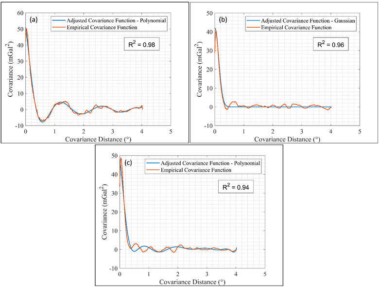
In the context of the Remove step, Table 1 presents the R² values obtained by comparing the ACF with the ECF in each TOD tested. The best result is shown in blue in each TOD. For the case of TOD 300, the most adjusted ACF was the 10^th and 12^th order Polynomial functions. In order to avoid overparameterization problems, the 10^th Polynomial was chosen. On the other hand, for TOD 500 the most appropriate ACF was the Gaussian function. Using TOD 760, both the Gaussian and the 12^th order polynomial functions proposed the best results. The polynomial function was here chosen as an empirical option. In almost all cases, the sine and Fourier polynomial functions presented the worst results, with all R² values below 0.70. Figure 4 shows the plots of the most appropriate ACFs.

Table 1:
R² values when comparing ACF with ECF in each TOD tested.

ACF	TOD 300	TOD 500	TOD 760
Exponential	0.83	0.90	0.85
Fourier	0.40	0.32	0.72
Gaussian	0.81	0.96	0.94
Hirvonen	0.80	0.93	0.90
Markov 2nd order	0.79	0.76	0.77
Polynomial sine	0.32	0.46	0.45
Reilly	0.76	0.93	0.91
Polynomial 10th order	0.98	0.93	0.92
Polynomial 12th order	0.98	0.95	0.94

Figure 4:
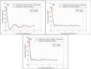
Plot of ACFs (line in blue) (a) 12^th order polynomial for TOD 300, (b) Gaussian for TOD 500, and (c) 12^th order polynomial for TOD 760, together with the respective ECF (line in orange).

To evaluate the omission and commission errors of the combined XGM2019, REQ_TOPO_2015, and ERTM2160 models, Root Mean Square Error (RMSE) values of the residual gravity anomalies were determined considering the different TDOs (Table 2). The values remained between 6.22 and 8.25 mGal. Disregarding errors in gravity and geodetic coordinates data, and considering the same omission error in all configurations, the configuration using a TDO of 760 proposed the smallest commission error, with a difference of 0.27 mGal in relation to the result obtained using a TDO of 500. These results point to lower commission error for the XGM2019 model compared to REQ_TOPO_2015 in the tested bandwidths.

Table 2:
Statistics of the total errors of the combined XGM2019, REQ_TOPO_2015, and ERTM2160 models. Units in mGal.

	TOD 300	TOD 500	TOD 760
RMSE	8.26	6.53	6.26

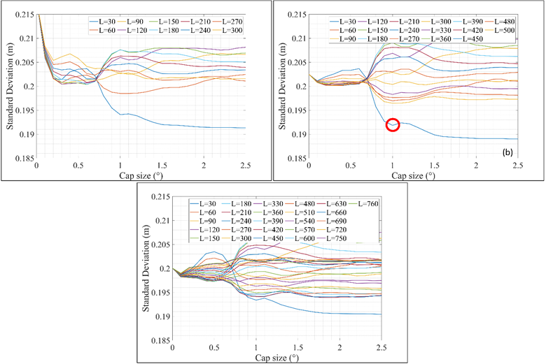
The optimal configuration can be identified from the graphs presented in Figures 5. The standard deviation values of the discrepancies, are on the ordinate axis. The abscissa contains the tested cap size values. The different curves are associated with the different tested L values. As can be seen, the optimal configuration was obtained with L = 30 and ψ ₀ = 2.5° and TOD 500, which proposed a standard deviation value of approximately 0.189 m. However, it should be remarked that, analyzing the graph in Figure 5(b), choosing ψ ₀ = 1° the standard deviation value is 0.192 m (circled in red), presenting a difference of 0.003 m. Taking into account that a smaller cap size is more interesting as it provides a smaller edge effect, the configuration L = 30 and ψ ₀ = 1° and TOD 500 was adopted to compute the PR_QG_A GQGM.

Figure 5:
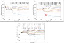
Graphs of standard deviation, cap size and L values for (a) TOD 300, (b) 500, and (c) 760.

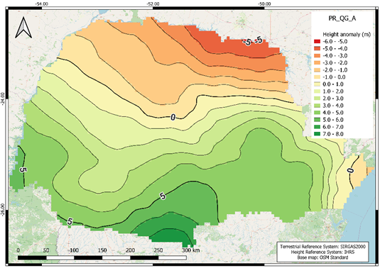
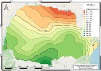
The PR_QG_A model is presented in Figure 6. It is apparent that, there is a smooth transition from negative to positive values in the central region of the state. In the North region, including the Northwest, North Central and Norte Pioneiro Paranaense and coastal region, values are negative, reaching up to -5.098 m in the Serra Geral Norte region. In the Center East, West, Southwest, Center-South, Southeast and metropolitan region of Curitiba the values are positive, reaching up to 7.693 m in the micro region of União da Vitória.

Figure 6:
PR_QG_A GQGM referenced to IHRS.

To analyze the quality of the PR_QG_A model, the height anomaly values (${{\zeta }_{IHRF}}_P$) were extracted from the model by bilinear interpolation for the positions of the 97 previously used GNSS/leveling stations. Their discrepancies in relation to the reference height anomaly values (${{\zeta }_{RN}}_P$), referenced to BVDI, were then calculated. In addition, for comparison and complementary validation purposes, the same process was carried out with the SAM_QGEOID2023 model available in the International Service for the Geoid (ISG) repository. However, before comparisons, the height anomaly values from SAM_QGEOID2023 were referenced to the IHRS, adding the second part of zero-degree term in Eq. (9) and using Eq. (11) to (16) and (18). This is because the model was computed using the concept of zero tide and using only the first part of zero-degree term in Eq. (9) (see details in Guimarães et al. 2025).

The statistical parameters of both set of discrepancies (Table 3) were calculated with and without subtracting the mean of the discrepancies. This with the purpose of to eliminate the biases associated with the difference in height references, and to evaluate the quality of the PR_QG_B model referenced to the BVDI. The means of the discrepancy values were here considered as local vertical translation parameters for the transformation between the IHRS and the BVDI. In the case of the PR_QG_A model, the value of 0.411 m was found closer to the value previously obtained by Sánchez and Sideris (2017). The difference of 0.021 m between the values is close to the uncertainty of 0.020 m estimated by the mentioned authors. The local parameter value obtained for SAM_QGEOID2023 is closer to the translation value obtained by Guimarães et al. (2025), with a difference of 0.010 m.

Table 3:
Statistics of the discrepancies before and after transformation to the BVDI. Units in m.

Parameter	PR_QG_A	SAM_QGEOID2023 referenced to the IHRS	PR_QG_B	SAM_QGEOID2023 referenced to the BVDI
Mean	0.411	0.348	0.000	0.000
Std-dev	0.199	0.197	0.199	0.197
Minimum	-0.442	-0.499	-0.853	-0.847
Maximum	0.889	0.790	0.478	0.442
RMSE	0.456	0.399	0.198	0.196

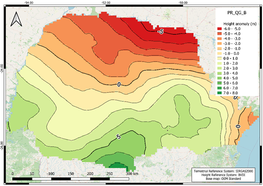
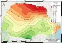
For both PR_QG models, the standard deviation value was 0.199 m. On the other hand, the RMSE value, after the transformation to BVDI, was almost three times smaller, close to the standard deviation value. Such a result is achieved by eliminating the influence of biases, which highlights the need to carry out the transformation for a more adequate assessment. After applying the local transformation parameter between the IHRS and BVDI in the PR_QG_A model, the PR_QG_B model was obtained (Figure 7).

Figure 7:
PR_QG_B GQGM referenced to BVDI.

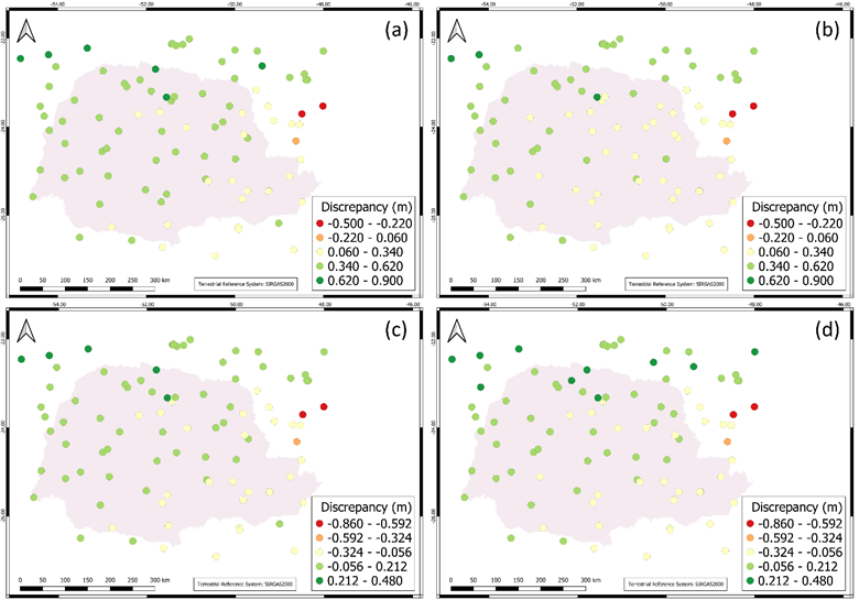
The spatial distribution of the height anomaly discrepancies for each model across all 97 GNSS/leveling stations is presented in Figure 8. It should be noted that the models were computed for the study area indicated in Section 2.1. Therefore, for the analyses and the calculation of the vertical translation parameter, discrepancies at GNSS/leveling stations located outside the state of Paraná were also taken into account.

Figure 8:
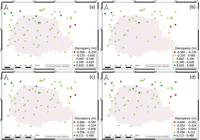
Spatial distribution of the height anomaly discrepancies at 97 GNSS/leveling stations for (a) PR_QG_A, (b) SAM_QGEOID2023 referenced to the IHRS, (c) PR_QG_B, and (d) SAM_QGEOID2023 referenced to the BVDI.

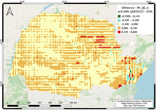
In comparison with the SAM_QGEOID2023 model, the standard deviation and RMSE values were practically the same, with differences of around 2 mm. Such a result indicates that the four solutions propose practically equivalent qualities. However, it is very important to highlight that the height anomaly values between the models differ by up to 0.707 m in certain regions, with 95% of absolute values below 0.264 m (Figure 9). A possible explanation for the result lies in the differences in computation methodology, models, and input data. Mean values equal to zero after transformations with local parameters indicate the elimination of biases.

Figure 9:
Differences between the PR_QG_A and SAM_QGEOID2023 models in the Paraná state - Brazil.

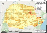
After applying the local transformation parameter of 0.348 m at the SAM_QGEOID2023 model, and comparing with the PR_QG_B model, it appears that the differences decrease slightly. In total, 95% of absolute values are below 0.220 m. However, difference absolute values of 0.770 m can still be verified.

4. Conclusions and outlooks

This study aimed to compute two GQGMs for the Paraná state, called PR_QG_A and PR_QG_B, referenced to IHRS and BVDI, respectively. A set of terrestrial and oceanic gravimetric data from different institutions was used, together with data obtained from the XGM2019, REQ_TOPO_2015 and ERTM2160 gravity field models. To provide residual height anomaly values, we used the GBVP scalar-free solution via Molodenskii series. Different TODs were tested, as well as an optimal configuration of modification degree of Stokes’ kernel and cap size, which has been identified from a set of point-wise iterative solutions for GNSS/leveling co-location stations. Using the optimal configuration, the PR_QG_A model was computed.

The model was evaluated against the same reference data from GNSS/leveling co-location stations. Using the mean value of the discrepancies as a local vertical translation parameter between IHRS and BVDI the PR_QG_B model was obtained. The results show that the precision of the both models is 0.199 m. For additional validation purposes, the SAM_QGEOID2023 model was also evaluated. Their precision is practically the same as the computed GQGMs. However, differences in height anomaly values in relation to the PR_QG_A model can be up to 0.707 m in some regions. Comparing the PR_QG_B model with the SAM_QGEOID2023 model referenced to the BVDI, the differences decrease slightly. However, absolute values of more than 0.75 m can still be verified. It is worth noting that, the models differ in terms of input data, TDO, RTM technique, type of GBVP solution, Stokes Integral solution, cap size, and modification degree of Stokes’ kernel.

Since only one local vertical translation transformation parameter was used here, possible systematic effects of inclination and scale factor were not modeled. Therefore, transformation with functional mathematical models using more parameters is recommended. It is also recommended to use clustering techniques to estimate regional/local parameters for sub-regions in the state, and thus increase the quality of the hybrid model, as done by Delgado and Rodrigues (2023) and Rodrigues et al. (2024).

Both computed models will be submitted to the ISG repository so that users can use them for free. Later versions of these models will include improvements such as numerical integration with Gauss-Legendre quadrature, ellipsoidal correction, spectral power density analysis for more adequate TOD determination and, additional GNSS/leveling co-location stations data.

ACKNOWLEDGEMENT

The authors would like to thank the National Council for Scientific and Technological Development (CNPq) for the financial support provided through Scientific Initiation scholarships. We also thank the Office of the Pro-Rector for Research and Graduate Studies (PRPPG) of the Federal University of Paraná (UFPR), specifically the Coordination of Scientific Research and Technological Development, for the financial support granted under call 04/2023. Further thanks are extended to the UFPR Graduate Program in Geology (Bárbara Dressel, Luiz Gustavo Castro, and Renata Zanella) and to Prof. Denizar Blitzkow for providing part of the gravimetric data used in this research.

REFERENCES

• Abdalla, A. and Ferreira, V. (2022) A semi-vectorized and relationally-operated algorithm for fast geoid computation using Stokes’s integration. Earth Science Informatics, 15 June, pp. 2017-2029. https://doi.org/10.1007/s12145-022-00822-7
  » https://doi.org/https://doi.org/10.1007/s12145-022-00822-7
• Andersen, O. B., Rose, S. K., Abulaitijiang, A., Zhang, S. and Fleury, S. (2023) The DTU21 global mean sea surface and first evaluation. Earth System Science Data, 15 (9) September, pp. 4065-4075. https://doi.org/10.5194/essd-15-4065-2023
  » https://doi.org/https://doi.org/10.5194/essd-15-4065-2023
• Blitzkow, D., Matos, A. C. O. C., Machado, W. C., Nunes, M. A., Lengruber, N. V., Xavier, E. M. L., Fortes, L. P. S. (2016). MAPGEO2015: the New Geoidal Undulation Model of Brazil. Revista Brasileira de Cartografia, 68 (10) November, pp. 1873-1884. https://doi.org/10.14393/rbcv68n10-44289
  » https://doi.org/https://doi.org/10.14393/rbcv68n10-44289
• Claessens, S. J. and Filmer, M. S., (2020) Towards an International Height Reference System: insights from the Colorado geoid experiment using AUSGeoid computation methods. Journal of Geodesy, 94 (52) May, pp. 1432-1394. https://doi.org/10.1007/s00190-020-01379-3
  » https://doi.org/https://doi.org/10.1007/s00190-020-01379-3
• Delgado, R. E. and Rodrigues, T. L. (2023) Linkage of normal heights obtained from GNSS and refined XGM2019 GGM to brazilian vertical data using different approaches. Anuário do Instituto de Geociências, 46 January, pp. 1-14. https://doi.org/10.11137/1982-3908_2023_46_51121
  » https://doi.org/https://doi.org/10.11137/1982-3908_2023_46_51121
• Drewes, H., Kuglitsch, F., Adám, J., Rózsa, S. (2016) The geodesist’s handbook 2016. Journal of Geodesy , 90 September, pp. 907-1205. https://doi.org/10.1007/s00190-016-0948-z
  » https://doi.org/https://doi.org/10.1007/s00190-016-0948-z
• Duquenne, H., Everaerts, M. and Lambot, P. (2005) Merging a Gravimetric Model of the Geoid with GPS/Levelling data: an Example in Belgium. In: Jekeli, C., Bastos, L., Fernandes, J. (eds) Gravity, Geoid and Space Missions International Association of Geodesy Symposia, vol 129. Springer, Berlin, Heidelberg. https://doi.org/10.1007/3-540-26932-0_23
  » https://doi.org/https://doi.org/10.1007/3-540-26932-0_23
• Ekman, M. (1989) Impacts of geodynamic phenomena on systems for height and gravity. Bulletin Géodésique, 63 (3), pp. 281-296. https://doi.org/10.1007/BF02520477
  » https://doi.org/https://doi.org/10.1007/BF02520477
• Foroughi I, Vaníček P, Novák P, Kingdon RW, Sheng M, Santos MC (2017) Optimal combination of satellite and terrestrial gravity data for regional geoid determination using Stokes-Helmert’s method, the Auvergne test case. In: Marti U (ed) International Symposium on Gravity, Geoid and Height Systems 2016 IAG Symposia, vol 148. Springer, Cham, pp 37-43. https://doi.org/10.1007/1345_2017_22
  » https://doi.org/https://doi.org/10.1007/1345_2017_22
• Grombein, T., Seitz, K. and Heck, B. (2016) The rock-water-ice topographic gravity field model RWI_TOPO_2015 and its comparison to a conventional rock-equivalent version. Surveys in Geophysics, 37 (5) June, pp. 937-976. https://doi.org/10.1007/s10712-016-9376-0
  » https://doi.org/https://doi.org/10.1007/s10712-016-9376-0
• Guimarães, G. N., de Matos, A. C. O. C., Blitzkow, D. and de Almeida, F. G. V. (2025) High-resolution regional gravity field modeling to connect the local vertical systems in South America to the IHRF. Earth, Planets and Space, 77 (98) July, pp. 1-26. https://doi.org/10.1186/s40623-025-02226-5
  » https://doi.org/https://doi.org/10.1186/s40623-025-02226-5
• Heiskanen, W. A. (1967) Physical geodesy: [by] Weikko A. Heiskanen [and] Helmut Moritz San Francisco: W.H. Freeman.
• Hirt, C. and Kuhn, M. (2014) Band-limited topographic mass distribution generates full-spectrum gravity field: gravity forward modeling in the spectral and spatial domains revisited. Journal of Geophysical Research: Solid Earth, 119 (4) March, pp. 3646-3661. https://doi.org/10.1002/2013JB010900
  » https://doi.org/https://doi.org/10.1002/2013JB010900
• International Association of Geodesy. (2019) Resolution 3: Establishment of the International Height Reference Frame (IHRF). Montreal, Canada: IAG.
• Instituto Brasileiro de Geografia e Estatística. (2022) Model for converting geometric altitudes (given by GNSS) into physical altitudes (compatible with the SGB´s Vertical Datum) [Online]. Available from: <https://www.ibge.gov.br/en/geosciences/digital-surface-models/digital-surface-models/31312-model-to-convert-altitudes-hgeohnor2020modeloconversaoaltitudesgeometricasgnss-datumverticalsgb.html?=&t=sobre> [Accessed 4 December 2025].
  » https://www.ibge.gov.br/en/geosciences/digital-surface-models/digital-surface-models/31312-model-to-convert-altitudes-hgeohnor2020modeloconversaoaltitudesgeometricasgnss-datumverticalsgb.html?=&t=sobre
• MATLAB (2024) Vectorization [Online]. Available from: <Available from: https://www.mathworks.com/help/matlab/matlab_prog/vectorization.html > [Accessed 4 December 2025].
  » https://www.mathworks.com/help/matlab/matlab_prog/vectorization.html
• Moritz, H. (2000) Geodetic Reference System 1980. Journal of Geodesy , 74 March, pp. 128-133. https://doi.org/10.1007/s001900050278
  » https://doi.org/https://doi.org/10.1007/s001900050278
• Padilha, T. K., Rodrigues, T. L., Jaramillo, A. G. S. (2026) Quasi-geoid modelling using a fixed GBVP solution based on Brovar series in the Colorado Experiment area. Geodesy and Geodynamics (in press). https://doi.org/10.1016/j.geog.2026.01.005
  » https://doi.org/https://doi.org/10.1016/j.geog.2026.01.005
• Rodrigues, T. L. and Cagido, A. C. F. (2024) Uso del análisis de cluster en el cálculo de modelo de cuasi geoide híbrido. In: SIRGAS Symposium 2024, Bogotá, Colombia. Available from: <https://sirgas.ipgh.org/wp-content/uploads/2025/03/Uso-del-analisis-de-cluster-en-el-calculo-de-modelo-de-cuasi-geoide-hibrido-_Tiago-Lima-Rodrigues.pdf>
  » https://sirgas.ipgh.org/wp-content/uploads/2025/03/Uso-del-analisis-de-cluster-en-el-calculo-de-modelo-de-cuasi-geoide-hibrido-_Tiago-Lima-Rodrigues.pdf
• Sánchez, L. and Sideris, M. G. (2017) Vertical datum unification for the International Height Reference System (IHRS). Geophysical Journal International, 209 (2) May, pp. 570-586. https://doi.org/10.1093/gji/ggx025
  » https://doi.org/https://doi.org/10.1093/gji/ggx025
• Sánchez, L., Ågren, J., Huang, J., Wang, Y. M., Mäkinen, J., Pail, R., Barzaghi, R., Vergos, G. S., Ahlgren, K., Liu, Q. (2021) Strategy for the realisation of the International Height Reference System (IHRS). Journal of Geodesy , 95 (33) February, pp. 1-33. https://doi.org/10.1007/s00190-021-01481-0
  » https://doi.org/https://doi.org/10.1007/s00190-021-01481-0
• United Nations. (2015) A/RES/69/266 - Resolution adopted by the General Assembly on 26 February 2015. 69/266. A global geodetic reference frame for sustainable development. New York, US: UN.
• Wang, Y. M. et al. (2021) Colorado geoid computation experiment: overview and summary. Journal of Geodesy , 95 (127) November, pp. 1-21. https://doi.org/10.1007/s00190-021-01567-9
  » https://doi.org/https://doi.org/10.1007/s00190-021-01567-9
• Wenzel, H. G. (1985) Hochauflösende Kugelfunktionsmodelle für das Gravitationspotential der Erde. Wissenschaftliche Arbeiten der Fachrichtung Vermessungswesen der Universität Hannover, Nr. 137, Hannover, Germany.
• Wong, L., Gore, R. (1969) Accuracy of Geoid Heights from Modified Stokes Kernels. Geophysical Journal International , 18 (1) September, pp. 81-91. https://doi.org/10.1111/j.1365-246X.1969.tb00264.x
  » https://doi.org/https://doi.org/10.1111/j.1365-246X.1969.tb00264.x
• Zingerle, P. et al. (2020) The combined global gravity field model XGM2019e. Journal of Geodesy , 94 (66) July, pp. 1-12. https://doi.org/10.1007/s00190-020-01398-0
  » https://doi.org/https://doi.org/10.1007/s00190-020-01398-0

• DATA AVAILABILITY
  The codes and dataset that support the findings of this work are available from the corresponding author on request.

• Edited by
  Silvana Philippi Camboim and Daniele Barroca Marra Alves.

Data availability

The codes and dataset that support the findings of this work are available from the corresponding author on request.

Publication Dates

• Publication in this collection
  22 June 2026
• Date of issue
  2026

History

• Received
  05 Dec 2025
• Accepted
  06 Apr 2026