Radial basis functions applied to the spatial interpolation of categorical variables: effect of parameters, neighborhood and number of categories

Abstract:

Spatial interpolation of categorical variables is a challenge in geosciences and other applied fields, especially when attempting to predict categories in unsampled locations. In this study, we evaluated the performance of generalized multiquadric radial basis functions (GM RBFs) in the interpolation of categorical variables, considering different parameters (a and b), local neighborhoods (k neighbors), and number of categories (2, 4, and 8). Simulated scenarios with 200 points in a two-dimensional grid were used to control the distribution of categories, allowing the comparison of 12 versions of the GM RBFs using metrics such as accuracy, mean of F1 score, and global variance (GV). The results showed that the best performance occurred for local neighborhoods (k = 10), with a parameter values ​​close to zero. For two or four categories, b = 0 presented the best results, while for eight categories, b = -1 was more efficient. Increases in the number of categories increased GV and reduced accuracy, demonstrating greater complexity in spatial prediction. The results reinforce the importance of adjusting RBF parameters and the number of neighbors according to the context, in addition to highlighting the impact of the number of categories and data imbalance on the interpolation efficiency.

Keywords:
Spatial statistics; Spatial autocorrelation; Multiquadric equations; Mapping

1. Introduction

Spatial interpolation methods have been widely used to generate maps of the spatial distribution of variables, by predicting values at unsampled locations from collected data. There are many approaches to spatial interpolation, including the kriging, the inverse distance weighted (IDW), the nearest neighbor, and the multiquadric equation methods (Yamamoto and Landim 2013).

Multiquadric equations allow the interpolation of both quantitative (Yamamoto 2002) and qualitative variables (Yamamoto et al. 2012). Interest in studying qualitative (or categorical) variables in a spatial context is quite common (Costa et al 2019; Jorreto-Zaguirre et al 2020; Cima et al. 2021; Mancell and Deutsch 2021; Zhang, Li, Zhang 2021; Dinda, Samanta and Chakravarty 2022; Madani, Maleki and Soltani-Mohammad 2022; Minniakhmetov and Dimitrakopoulos 2022; Sanchez and Deutsch 2022; Tsekeris, Zhang and Deutsch 2023; Zhang et al 2023; Zhang et al 2024; Santos et al 2025).

The multiquadric equations method uses radial basis functions (RBFs) to generate weights from interpolation distances. Spatial interpolation using RBFs emerged in the 1970s with the proposal of using multiquadric equations to represent surfaces from data points (Hardy 1971). According to Yamamoto et al. (2012), interpolation by multiquadric equations is more efficient for mapping qualitative data, compared to traditional methods, such as kriging. However, sequential indicator simulation (Yamamoto et al. 2015; Jorreto-Zaguirre et al 2020; Madani 2022; Madani, Maleki and Soltani-Mohammad 2022; Mizuno and Deutsch 2022), distance-based methods (Silva 2015; Rolo et al. 2017) or k-nearest neighbors (KNN) algorithms (Grossenbacher, 2018; Santos et al 2025) are also good alternatives for mapping categorical data.

Multiquadric equations were used by Costa et al. (2019) to map pest occurrence categories in irrigated rice crops in southern Brazil. Cima et al. (2021) used multiquadric equations to interpolate static warehouse capacity categories in an agricultural season in the state of Paraná. From a theoretical perspective, Yamamoto et al. (2014) evaluated post-processing methods to reduce uncertainty in the prediction of categorical variables, with multiquadric equations, in Geology.

However, there are still significant gaps in the literature regarding which RBF is the most efficient for different numbers of categories. The lack of comprehensive comparative studies evaluating the relative performance of RBFs in different interpolation scenarios limits the ability of researchers and practitioners to make informed choices. Thus, the objective of the current work is to evaluate the performance of generalized multiquadric radial basis functions (GM RBFs), varying the parameters and the number of neighbors in the interpolation of categorical variables with different numbers of categories (2, 4, and 8 categories), based on criteria such as the accuracy and agreement between the observed values and the predicted values. Based on this analysis, we seek to provide clear guidelines for choosing the most appropriate RBF, contributing both to the theoretical advancement of the area and to more efficient and precise practical applications.

This study goes beyond previous works by providing a comparative evaluation of GM RBFs performance under different parameter configurations, neighborhood sizes, numbers of categories and unbalanced categories, aiming to establish practical guidelines for categorical spatial interpolation.

2. Spatial interpolation of categorical variables using multiquadric equations

According to Yamamoto et al. (2012), RBFs are a promising method for interpolating categorical variables. The proposed methodology transforms categorical variables into indicator functions, which are interpolated and then retransformed, with emphasis on the use of the multiquadric kernel, which provides non-singular matrices and high precision, as evidenced by Franke (1982). Furthermore, an important difference is the inclusion of interpolation variance, which allows mapping zones of uncertainty in transitions between categories (Yamamoto et al. 2012).

To perform spatial interpolation, first, the categorical variable Z, with K categories (C ₁ , C ₂ , …C _K ), is transformed into K indicator variables as follows:

$Z\left(x_i\right)=\left\{\begin{array}{c}{C}_1,\to I\left(x_i;1\right)=\left\{\begin{array}{c}0,ifZ\left(x_i\right)\ne C_1\\ 1,ifZ\left(x_i\right)=C_1\end{array}\right.\\ C_2,\to I\left(x_i;2\right)=\left\{\begin{array}{c}0,ifZ\left(x_i\right)\ne C_2\\ 1,ifZ\left(x_i\right)=C_2\end{array}\right.\\ ⋮\\ C_K,\to I\left(x_i;K\right)=\left\{\begin{array}{c}0,ifZ\left(x_i\right)\ne C_K\\ 1,ifZ\left(x_i\right)=C_K\end{array}\right.\end{array}\right.$

The k-th indicator variable is defined as:

$I\left(k\right)=\left\{\begin{array}{c}1,ifthek-thcategoryisobserved\\ 0,ifthek-thcategoryisnotobserved\end{array}\right.$

The indicator variable of the k-th category [I(k)] has expectation and variance given by, respectively:

$E\left(I\left(k\right)\right)=p_k$ (1)

and

$V\left(I\left(k\right)\right)=p_k\left(1-p_k\right)$ (2)

In which p _k is the probability of occurrence of the k-th category.

Subsequently, interpolation is performed, using multiquadric equations, for each of the K indicator variables, at point x ₀ , using the following expression (Yamamoto et al. 2012; Yamamoto and Landim 2013):

${I^{*}}_{MQ}\left(x_0;k\right)=\sum _{i=1}^n{w}_i.I\left(x_i;k\right)$ (3)

in which I(xi; k) is the value of the indicator variable of the k-th type (k = 1, 2, ..., K), at point x _i and w _i is the i-th weight (i = 1, 2, ..., n). The weights w _i must satisfy the condition $\sum _{i=1}^n{w}_i=1$.

The weights w _i are obtained from the solution of a system of linear equations in the form (Yamamoto and Landim 2013):

$\left\{\begin{array}{c}\sum _{j=1}^n{w}_j\varphi \left(x_i-x_j\right)+\mu =\varphi \left(x_i-x_0\right),fori=1,2,\dots ,n\\ \sum _{j=1}^n{w}_j=1\end{array}\right.$ (4)

ϕ(.) is the radial basis function and µ is the Lagrange multiplier.

To avoid negative weights, the algorithm proposed by Rao and Journel (1997) is implemented, in which a constant equal to the module of the largest negative weight is added to all weights, which are then recalculated to result in a sum equal to 1.

The RBFs most commonly used in the literature, according to Yamamoto (2002), are presented below:

${\varphi \left(h\right)}_{Linear}=\left|h\right|$ (5)

${\varphi \left(h\right)}_{Cubic}={\left|h\right|}^3$ (6)

${\varphi \left(h\right)}_{GeneralizedMultiquadric}={\left(a+{\left|h\right|}^2\right)}^{\frac{2b+1}{2}}$ (7)

${\varphi \left(h\right)}_{Splines}={\left|h\right|}^{2}log\left|h\right|$ (8)

${\varphi \left(h\right)}_{Gaussian}=exp\left(-c{\left|h\right|}^2\right)$ (9)

in which h is the Euclidean distance between two points in two-dimensional space, and a (a ≥ 0), b (b = -1, 0, 1, …) and c (c > 0) are constants.

An advantage of interpolation using multiquadric equations is that it guarantees the property of total probability, since $\sum _{k=1}^K{I^{*}}_{MQ}\left(x_0;k\right)=1$ (Yamamoto and Landim 2013).

Finally, the predicted category at point x ₀ , called k _max , is obtained by $Z\left(x_0\right)=C_{k_{máx}}$, since ${I^{*}}_{MQ}\left(x_0;k_{max}\right)=max\left({I^{*}}_{MQ}\left(x_0;k\right),k=1,2,\dots ,K\right)$. This prediction is obtained based on the suggestion of Teng and Koike (2007), in which the highest value of the indicator is interpreted as the most likely categorical type.

It is possible to show that the linear and cubic RBFs are particular cases of the generalized multiquadric RBF, with a = 0, when we have b = 0 and b = 1, respectively. In the case of considering a = 0 and b = 0, we have:

$\varphi \left(h\right)={\left(a+{\left|h\right|}^2\right)}^{\frac{2b+1}{2}}={\left(0+{\left|h\right|}^2\right)}^{\frac{2\left(0\right)+1}{2}}={\left({\left|h\right|}^2\right)}^{\frac{1}{2}}=\left|h\right|$

While, in the case where a = 0 and b = 1, we have:

$\varphi \left(h\right)={\left(a+{\left|h\right|}^2\right)}^{\frac{2b+1}{2}}={\left(0+{\left|h\right|}^2\right)}^{\frac{2\left(1\right)+1}{2}}={\left({\left|h\right|}^2\right)}^{\frac{3}{2}}={\left|h\right|}^3$

Thus, it can be seen that the results obtained by linear RBF or by GM RBF with a = 0 and b = 0 are the same. Similarly, the results of cubic RBF and GM RBF with a = 0 and b = 1 are the same.

3. Material and Methods

3.1 Simulation of scenarios

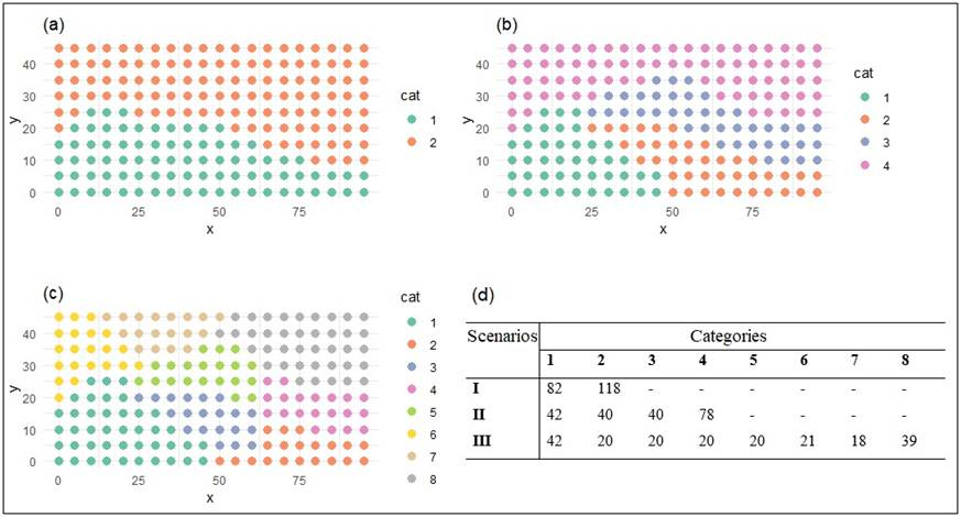
To compare the radial basis functions, three simulated scenarios are proposed. The first scenario considers two categories, the second scenario has four categories, and the third scenario consists of eight categories. In all scenarios, there are 200 observations in two-dimensional space. Figure 1 shows the locations of the simulated samples and the number of observations in the categories for each of the three scenarios.

Figure 1:
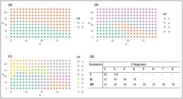
Simulated scenarios with two categories (a), four categories (b), and eight categories (c), and the number of points for the categories in the scenarios (d).

3.2 Evaluation criteria

The data in each scenario were separated into a training set (160 observations => 80%) and a validation set (40 observations => 20%). Thus, the RBFs were trained with 160 observations and validated with 40 observations.

In the current study, generalized multiquadric (GM) RBFs will be considered. To compare the RBFs, the following values for the constants a and b will be considered: a = (0, 5, 50, 500); b = (-1, 0, 1). Thus, the generalized multiquadric RBFs will have 12 versions.

To compare the RBFs, three criteria are used based on the validation data:

1. Accuracy value obtained from the confusion matrix.

2. F1 (mean) score obtained from the confusion matrix.

3. Global variance.

The confusion matrix is obtained through a two-way matrix, in which the rows indicate the observed categories in each scenario and the columns indicate the categories predicted by interpolation in each scenario.

Accuracy is obtained by the expression:

$accuracy=\frac{\sum _{ii}{n}_{ii}}{n}$ (10)

in which n _ii is the element of the main diagonal of the confusion matrix and $n=\sum _{ij}{n}_{ij}$ is the total number of elements in the confusion matrix. Accuracy ranges from 0 to 1; the closer to 1, the more accurate the prediction by spatial interpolation.

The l-th F1 score is obtained from the expression:

${F1}_l=\frac{2.{precision}_j.{recall}_i}{{precision}_j+{recall}_i}$ (11)

in which the j-th precision value is ${precision}_j=\frac{n_{ii}}{C_j}$, and the i-th recall value is ${recall}_i=\frac{n_{ii}}{R_i}$. R _i is the total number of elements in the i-th row and C _j is the total number of elements in the j-th column of the confusion matrix.

The mean of F1 is obtained from the expression:

$MeanofF1=\frac{\sum _{l=1}^L{F1}_l}{L}$ (12)

in which L = I = J (number of rows or number of columns).

The global variance (GV) is given by (Kader and Perry 2007):

$GV=\sum _{k=1}^K{\widehat{p}}_k\left(1-{\widehat{p}}_k\right)$ (13)

in which ${\widehat{p}}_k=\frac{n_k}{m}$ is the proportion of interpolated points of the k-th category, n _k is the number of interpolated points of the k-th category, and m is the total number of points in the interpolation grid.

Finally, the GM RBF that presents the best values for criteria i), ii), and iii) will be considered the most efficient. All routines were written in R language. (R Core Team 2021).

3.3 Application to real data

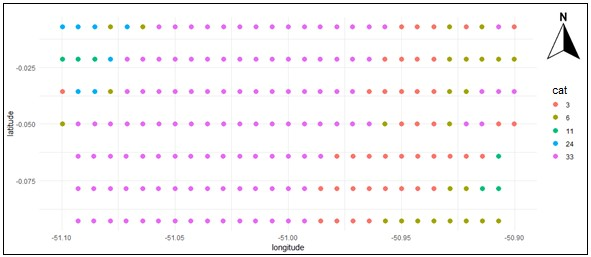
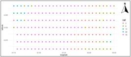
To demonstrate the applicability of spatial interpolation with the most efficient GM RBF, MapBiomas data are used to model the categorical variable land cover. The data are available in the MapBiomas platform (https://brasil.mapbiomas.org/), Brazil. A total of 197 georeferenced samples of land cover classes were collected in a regular grid for the year 2024 in an area near the city of Macapá - AP, Brazil. There were 42 samples from class 3 (forest formation), 25 samples from class 6 (flooded forest), 6 samples from class 11 (flooded field), 7 samples from class 24 (urban area), and 117 samples from class 33 (water). Figure 2 shows the sampling grid of land cover classes.

Figure 2:
Sampling grid of land cover classes, in the year 2024, in the Macapá region - AP, Brazil.

4. Results and Discussion

4.1 Analysis of the simulated scenarios

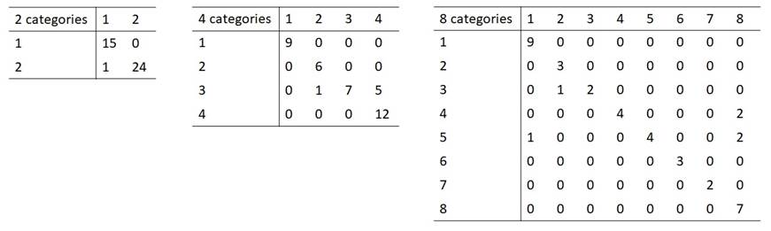
Table 1 presents the accuracy, and mean of F1 values for the 12 versions of GM RBFs for 2, 4, and 8 categories. The best performance, in the first scenario (with 2 categories), is obtained for the GM RBFs with any a and b and for k = 10 neighbors (local neighborhood), having the highest accuracy and mean of F1 values. A mean of F1 value of 0.974 (based on the confusion matrix for 2 categories in Figure 3, Appendix) indicates a similarity between the observed values and the values predicted by spatial interpolation.

It can be identified that only one sample point was not correctly interpolated (accuracy=39/40=0.975), demonstrating the efficiency of the method in the simplest situation of interpolation of categorical variables (2 categories).

Table 1:
Accuracy, and Mean of F1 for the 12 versions of the generalized multiquadric radial basis functions, for k = 10 and k = 100 neighbors, in the spatial interpolation for 2, 4, and 8 categories in the validation set.

Scenarios	Metrics	a	b	k = 100 (Global)	k = 10 (Local)
I (2 categories)	Accuracy	0	-1	0.875	0.975
	Mean of F1	0	-1	0855	0.974
	Accuracy	0	0	0.950	0.975
	Mean of F1	0	0	0.947	0.974
	Accuracy	0	1	0.850	0.975
	Mean of F1	0	1	0.835	0.974
	Accuracy	5	-1	0.950	0.975
	Mean of F1	5	-1	0.947	0.974
	Accuracy	5	0	0.875	0.975
	Mean of F1	5	0	0.860	0.974
	Accuracy	5	1	0.825	0.975
	Mean of F1	5	1	0.804	0.974
	Accuracy	50	-1	0.850	0.975
	Mean of F1	50	-1	0.829	0.974
	Accuracy	50	0	0.825	0.975
	Mean of F1	50	0	0.804	0.974
	Accuracy	50	1	0.825	0.975
	Mean of F1	50	1	0.804	0.974
	Accuracy	500	-1	0.825	0.975
	Mean of F1	500	-1	0.804	0.974
	Accuracy	500	0	0.825	0.975
	Mean of F1	500	0	0.804	0.974
	Accuracy	500	1	0.825	0.975
	Mean of F1	500	1	0.804	0.974
II (4 categories)	Accuracy	0	-1	0.425	0.800
	Mean of F1	0	-1	0.367	0.811
	Accuracy	0	0	0.775	0.850
	Mean of F1	0	0	0.791	0.863
	Accuracy	0	1	0.600	0.800
	Mean of F1	0	1	0.587	0.816
	Accuracy	5	-1	0.800	0.825
	Mean of F1	5	-1	0.816	0.839
	Accuracy	5	0	0.600	0.850
	Mean of F1	5	0	0.587	0.863
	Accuracy	5	1	0.550	0.800
	Mean of F1	5	1	0.519	0.816
	Accuracy	50	-1	0.600	0.825
	Mean of F1	50	-1	0.587	0.845
	Accuracy	50	0	0.525	0.825
	Mean of F1	50	0	0.497	0.835
	Accuracy	50	1	0.500	0.775
	Mean of F1	50	1	0.473	0.793
	Accuracy	500	-1	0.475	0.825
	Mean of F1	500	-1	0.446	0.835
	Accuracy	500	0	0.475	0.800
	Mean of F1	500	0	0.446	0.811
	Accuracy	500	1	0.450	0.775
	Mean of F1	500	1	0.415	0.793
III (8 categories)	Accuracy	0	-1	0.400	0.850
	Mean of F1	0	-1	0.145	0.864
	Accuracy	0	0	0.650	0.825
	Mean of F1	0	0	0.584	0.813
	Accuracy	0	1	0.400	0.800
	Mean of F1	0	1	0.145	0.805
	Accuracy	5	-1	0.775	0.825
	Mean of F1	5	-1	0.755	0.813
	Accuracy	5	0	0.450	0.825
	Mean of F1	5	0	0.296	0.813
	Accuracy	5	1	0.400	0.825
	Mean of F1	5	1	0.145	0.848
	Accuracy	50	-1	0.400	0.850
	Mean of F1	50	-1	0.145	0.866
	Accuracy	50	0	0.400	0.800
	Mean of F1	50	0	0.145	0.798
	Accuracy	50	1	0.400	0.775
	Mean of F1	50	1	0.145	0.780
	Accuracy	500	-1	0.400	0.800
	Mean of F1	500	-1	0.145	0.798
	Accuracy	500	0	0.400	0.800
	Mean of F1	500	0	0.145	0.798
	Accuracy	500	1	0.400	0.775
	Mean of F1	500	1	0.145	0.780

In the second scenario (with 4 categories), the best performance is obtained for the GM RBF with a = 0 or a = 5 and b = 0, having an accuracy of 0.850 and mean of F1 value equal to 0.863 (based on the confusion matrix for 4 categories in Figure 3, Appendix), showing high similarity between the observed and predicted values.

Considering GM RBF with a = 0 and b = 0, for k = 10 neighbors, in the spatial interpolation of the variable with 4 categories, only 6 points were interpolated into the wrong categories. The 0.850 accuracy represents 87.18% of the 0.975 accuracy of the first scenario, indicating that doubling the categories of the variable results in a 12.82% decrease in spatial interpolation accuracy.

In the scenario III (with 8 categories), the best performance is obtained for the GM RBF with a = 0 or a = 50 and b = -1, generating accuracy value of 0.850 (based on the confusion matrix for 8 categories in Figure 3, Appendix). The means of F1 are 0.866 and 0.864 for the GM RBF with a = 50 and a = 0, respectively, and b = -1, indicates a high similarity between the observed values and the values predicted by spatial interpolation.

For GM RBF with a = 0 and b = -1, for k = 10 neighbors, only 6 points were interpolated into the wrong categories. It can be seen that, when increasing the number of categories of the variable from 2 to 8, there is a 12.82% decrease in the accuracy of spatial interpolation. However, when increasing from 4 to 8 categories, there is no decrease in accuracy.

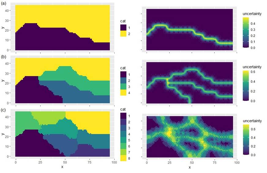
Figure 4 shows the spatial interpolations, and associated uncertainties, for the three simulated scenarios. The associated uncertainty was obtained by $1-maximum\left(\widehat{p}\right)$. An increase in uncertainty (variability) is evident as the number of categories to be interpolated increases. Interpolation at the boundaries between categories becomes less accurate for more categories.

Cartographic products (interpolation maps) discussed without explicit information on uncertainty can lead to misinterpretations and convey a false sense of accuracy (Lindi et al. 2024; Adediran et al. 2025). Thus, presenting the associated uncertainty allows for quantifying the local ambiguity of the classification, contributing to a more accurate interpretation of the results.

Figure 4:
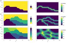
Maps of spatial interpolations for 2 categories [a = 0, b = 0, k = 10] (a), 4 categories [a = 0, b = 0, k = 10] (b), and 8 categories [a = 0, b = -1, k = 10] (c), with associated uncertainties.

Yamamoto et al. (2012) and Costa et al. (2019) used GM RBFs with a = 0 and b = 0. Bayona et al. (2011) and Yamamoto et al. (2014) recommend using small values of a (close to zero), as these generate greater interpolation efficiency. These studies corroborate the findings of the current article, where MG RBFs with a = 0 showed good results. For 2 and 4 categories, b = 0 yielded better results, while for 8 categories, b = -1 yielded better results. This indicates that the same RBF will not necessarily be best in all scenarios and applications. However, in practice, it is more common to use b = 0 (Yamamoto et al. 2012; Yamamoto et al. 2014).

The best accuracy and mean of F1 results were obtained with k = 10 neighbors (local neighborhood) compared to k = 100 neighbors (global neighborhood). The use of a local neighborhood was also indicated as more appropriate by Yamamoto et al. (2014), who suggest using 4 to 12 neighbors in the interpolation.

It is important to note that the scenarios considered include some categories with different numbers of observations (unbalanced categories, as frequently observed in applications with real data), a fact that can harm spatial interpolations, which is still little explored in the literature with interpolations using RBFs. According to Yamamoto et al. (2012), categories with few observations can harm spatial modeling. Data imbalance is addressed, in the context of learning from data, most notably in He and Garcia (2009), who show that minority classes tend to demonstrate lower performance in predictions.

Furthermore, it is observed that the maximum values of accuracy and mean of F1 decrease as the number of categories increases, indicating that the efficiency of prediction by spatial interpolation tends to decrease for variables with many categories. This effect is consistent with observations in machine learning, where algorithms exhibit reduced performance for underrepresented classes in multiclass scenarios (He and Garcia 2009). However, further studies must be developed to identify how this efficiency decreases or which number of neighbors is more appropriate as the number of categories of variables to be interpolated increases.

Another important aspect is that global variance (GV) values, showed in Table 2 (Appendix), tend to increase as the number of categories of the variable increases, indicating greater heterogeneity and lower precision in spatial interpolation, as it becomes more difficult to separate more categories into neighboring areas. Thus, as GV increases, accuracy and the mean of F1 decrease.

Multiquadric equations may offer advantages for interpolating categorical data, particularly in situations where variogram modeling becomes unreliable. As highlighted by Yamamoto et al. (2012), a fundamental limitation of indicator kriging is the need to model a semivariogram for each category. When some categories are underrepresented, the corresponding indicator semivariograms may be poorly defined due to the limited number of data pairs, leading to unstable or unreliable estimates. In such cases, multiquadric approaches provide a practical alternative by avoiding the need for variogram modeling.

4.2 Spatial interpolation of the land cover

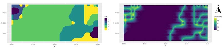
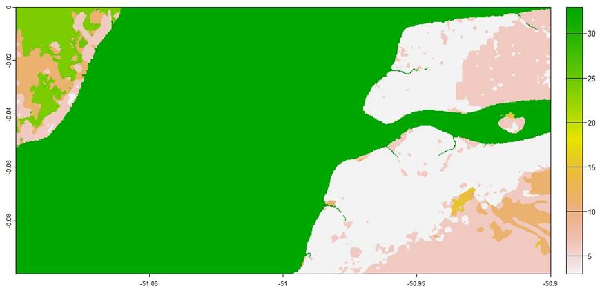
Figure 5 presents the predicted categories of land cover and associated uncertainties, using GM RBF with a = 0 and b = 0 for k = 10 neighbors (local neighborhood). There is a predominance of the classes water (code 33), forest formation (code 3), and flooded forest (code 6).

The uncertainty is greater in the transition regions between land cover categories. In addition, the average uncertainty was 0.12 and the maximum uncertainty was 0.74. Another important observation is that the land cover has unbalanced categories, with different amounts of data per category, a fact that can harm the efficiency of spatial interpolation.

Figure 5:
Spatial interpolation and associated uncertainty of land cover categories.

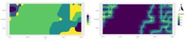
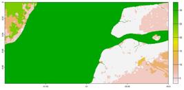
The application of the spatial interpolation method to MapBiomas data showed the maintenance of dominant spatial patterns, without the introduction of significant artificial fragmentation. The area of study is shown in Figure 6 (Appendix). Here, the intention was not to reassess performance, but to demonstrate the operability of the method in a real-world scenario with a complex spatial pattern.

Different spatial interpolation methods are applied to categorical data (Zhang, Li, Zhang 2021; Dinda, Samanta and Chakravarty 2022; Madani 2022; Madani, Maleki and Soltani-Mohammad 2022; Minniakhmetov and Dimitrakopoulos 2022; Zhang et al 2023; Zhang et al 2024), highlighting methodological challenges, and thus remaining a topic of constant discussion in the literature (Santos et al 2025).

Despite the contributions of this study, some limitations should be acknowledged. First, the simulated scenarios were based on regular sampling grids and relatively simple spatial structures, which may not fully represent the complexity of real-world datasets. Second, the application to real data was restricted to a single study area, which may limit the generalization of the results. Third, although the presence of unbalanced categories was observed and discussed, its effects on interpolation performance were not systematically evaluated. Future studies should address these aspects by considering more complex spatial patterns, different sampling designs, data with more categories, and a broader range of real datasets.

5. CONCLUSION

The current work evaluated the use of radial basis functions (RBFs) for the spatial interpolation of categorical variables in simulated scenarios and in land cover data from MapBiomas. The main objective was to identify the influence of the generalized multiquadric (GM) RBF parameters (a and b), number of neighbors (k), and number of categories of the variable, on the interpolation performance, considering metrics such as accuracy, F1-score, and global variance.

The results showed that GM RBFs with a = 0 performed best in all scenarios. The b parameter demonstrated behavior dependent on the number of categories: for two and four categories, b = 0 was most appropriate, while for eight categories, the best performance occurred with b = -1. In all cases, interpolation with local neighborhoods (k = 10 neighbors) outperformed global neighborhoods (k = 100), indicating that the choice of k is crucial to reduce errors and improve interpolation stability. Furthermore, we observed that the accuracy and mean of F1 decreased with increasing numbers of categories and global variances, highlighting the additional complexity imposed by greater category diversity.

The findings of the current study reinforce the potential of RBFs for spatial interpolation of categorical variables, highlighting the importance of adjusting the function parameters and number of neighbors according to the context. The results can guide professionals in geological mapping, soil classification, and environmental and climate applications that use categorical datasets, offering practical guidelines for applying the method to real data.

Future perspectives include expanding the analysis to scenarios with highly imbalanced categories, testing other RBFs, and comparing performance with other methods, such as indicator kriging, sequential indicator simulated, signed distance and machine learning methods.

ACKNOWLEDGMENT

We would like to thank the Federal University of Amapá for granting a scholarship from the Institutional Program for Scholarships for Initiation in Technological Development and Innovation (PIBITI UNIFAP) to the first author.

REFERENCES

• Adediran, E. et al. (2025) Toward Quantifying Interpolation Uncertainty in Set-Line Spacing Hydrographic Surveys. ISPRS International Journal of Geo-Information, 14. DOI: 10.3390/ijgi14020090.
  » https://doi.org/10.3390/ijgi14020090
• Bayona, V. et al. (2011) Optimal constant shape parameter for multiquadric based RBF-FD method. Journal of Computational. Physics, 230, pp.7384-7399. DOI 10.1016/j.jcp.2011.06.005.
  » https://doi.org/0.1016/j.jcp.2011.06.005
• Cima, E. G. et al. (2021) Forecasting Grain Production and Static Capacity of Warehouses Using the Natural Neighbor and Multiquadric Equations. AGRIS on-line Papers in Economics and Informatics, 13(3), pp.3-14. DOI 10.7160/aol.2021.130301.
  » https://doi.org/0.7160/aol.2021.130301
• Costa, H. S. et al. (2019) Mapping of spatiotemporal distribution of Tibraca limbativentris Stal (Hem.: Pentatomidae) inflooded rice crop in Southern Brazil. Revista Brasileira de Entomologia, 63, pp.205-211. DOI 10.1016/j.rbe.2019.04.001.
  » https://doi.org/0.1016/j.rbe.2019.04.001
• Dinda, K., Samanta, B. and Chakravarty, D. (2022) A v-transformed copula-based simulation model for lithological classification in an Indian copper deposit. Scientific Reports, 12. DOI: 1038/s41598-022-24233-2.
  » https://doi.org/1038/s41598-022-24233-2
• Franke, R. (1982) Scattered data interpolation: test of some methods. Mathematics of Computation, 38, pp.181-200. DOI 10.1090/s0025-5718-1982-0637296-4.
  » https://doi.org/10.1090/s0025-5718-1982-0637296-4
• Grossenbacher, T. (2018) Categorical Spatial Interpolation. Blog post Categorical Spatial Interpolation by Timo Grossenbacher. Retrieved from https://timogrossenbacher.ch/2018/03/categorical-spatial-interpolation-with-r/
  » https://timogrossenbacher.ch/2018/03/categorical-spatial-interpolation-with-r/
• Hardy, R. L. (1971) Multiquadric equations of topography and other irregular surfaces. Journal of Geophysical Research, 76, pp.1905-1915. DOI 10.1029/JB076i008p01905.
  » https://doi.org/10.1029/JB076i008p01905
• He, H. and Garcia, E. A. (2009) Learning from imbalanced data IEEE Transactions on Knowledge and Data Engineering DOI 10.1109/TKDE.2008.239.
  » https://doi.org/10.1109/TKDE.2008.239
• Jorreto-Zaguirre, S. et al. (2020) Stochastic Simulation of the Spatial Heterogeneity of Deltaic Hydrofacies Accounting for the Uncertainty of Facies Proportions. Frontiers in Earth Sciences, 8, pp.1-17. DOI: 10.3389/feart.2020.563122.
  » https://doi.org/10.3389/feart.2020.563122
• Kader, G. D. and Perry, M. (2007) Variability for categorical data. Journal of Statistics Education, 15. DOI 10.1080/10691898.2007.11889465.
  » https://doi.org/10.1080/10691898.2007.11889465
• Lindi, O. T. et al. (2024) Uncertainty Quantification in Mineral Resource Estimation. Natural Resources Research, 33, pp.2503-2526. DOI: 10.1007/s11053-024-10394-6.
  » https://doi.org/10.1007/s11053-024-10394-6
• Madani, N. (2022). Revisited Bayesian Sequential Indicator Simulation: Using a Log-Linear Pooling Approach. Mathematics, 10, pp.2-22. DOI: 10.3390/math10244669.
  » https://doi.org/10.3390/math10244669
• Madani, N., Maleki, M. and Soltani-Mohammadi, S. (2022) Geostatistical modeling of heterogeneous geo-clusters in a copper deposit integrated with multinomial logistic regression: An exercise on resource estimation. Ore Geology Reviews, 150. DOI: 10.1016/j.oregeorev.2022.105132.
  » https://doi.org/10.1016/j.oregeorev.2022.105132
• Mancell, S. A. and Deutsch, C. V. (2021) Geological boundary modeling with uncertainty using an indicator interpolated threshold approach. CIM Journal, 12, pp.95-104, DOI: 10.1080/19236026.2021.1945401.
  » https://doi.org/10.1080/19236026.2021.1945401
• Minniakhmetov, I. and Dimitrakopoulos, R. (2022) High-Order Data-Driven Spatial Simulation of Categorical Variables. Mathematical Geosciences, 54, pp.23-45. DOI: 10.1007/s11004-021-09943-z.
  » https://doi.org/10.1007/s11004-021-09943-z
• Mizuno, T. and Deutsch, C. (2022). Sequential Indicator Simulation (SIS) In Deutsch, J. L. (Ed.), Geostatistics Lessons. Retrieved from http://www.geostatisticslessons.com/lessons/sequentialindicatorsim
  » http://www.geostatisticslessons.com/lessons/sequentialindicatorsim
• R Core Team (2021) R: A language and environment for statistical computing R Foundation for Statistical Computing, Vienna, Austria. https://www.R-project.org/
  » https://www.R-project.org/
• Rao, S. E. and Journel, A. G. (1997) Deriving conditional distributions from ordinary kriging. In: Baafi, E.Y, Schofield, N. A, Geostatistics Wollongong ’96, Boston, Kluwer Academic Publishers, pp.92-102.
• Rolo, R. M. et al. (2017) Signed distance function implicit geologic modeling. REM - International Engineering Journal, 70(2), pp.221-229. DOI 10.1590/0370-44672016700146.
  » https://doi.org/10.1590/0370-44672016700146
• Sanchez, S. and Deutsch, C. V. (2022) Domain Delimitation with Radial Basis Functions In Deutsch, J. L. (Ed.), Geostatistics Lessons, 2022. Retrieved from http://www.geostatisticslessons.com/lessons/implicitrbf
  » http://www.geostatisticslessons.com/lessons/implicitrbf
• Santos, S. D. et al. (2025). Regional wind variability in the state of Rio Grande do Sul, Brazil. HOLOS, 7, pp.1-18. DOI: 10.15628/holos.2025.15955.
  » https://doi.org/10.15628/holos.2025.15955
• Silva, D. A. (2015) Signed Distance Function Modeling with Multiple Categories In Deutsch, J. L. (Ed.), Geostatistics Lessons, 2015. Retrieved from http://geostatisticslessons.com/lessons/signeddistancefunctions
  » http://geostatisticslessons.com/lessons/signeddistancefunctions
• Teng, Y. and Koike, K. (2007) Three-dimensional imaging of a geothermal system using temperature and geological models derived from a well-log dataset. Geothermics, 36, pp.518-538. DOI 10.1016/j.geothermics.2007.07.006.
  » https://doi.org/10.1016/j.geothermics.2007.07.006
• Tsekeris, G., Zhang, B. and Deutsch, C. V. (2023) Categorical Variable Distributions in Geostatistics In Deutsch, J. L. (Ed.), Geostatistics Lessons . Retrieved from http://www.geostatisticslessons.com/lessons/categoricaldists
  » http://www.geostatisticslessons.com/lessons/categoricaldists
• Yamamoto, J. K. (2002) Ore reserve estimation using radial basis functions. Revista do Instituto Geológico, São Paulo, 23(1), pp.25-38. DOI 10.5935/0100-929X.20020003.
  » https://doi.org/10.5935/0100-929X.20020003
• Yamamoto, J. K. and Landim, P. M. B. (2013) Geoestatística: conceitos e aplicações São Paulo: Oficina de Textos.
• Yamamoto, J. K. et al. (2012) Mapping an uncertainty zone between interpolated types of a categorical variable. Computers & Geosciences 40, pp.146-152. DOI 10.1016/j.cageo.2011.09.005.
  » https://doi.org/10.1016/j.cageo.2011.09.005
• Yamamoto, J. K. et al. (2014) Post-processing for uncertainty reduction in computed 3D geological models. Tectonophysics, 633, pp.232-245. DOI 10.1016/j.tecto.2014.07.013.
  » https://doi.org/10.1016/j.tecto.2014.07.013
• Yamamoto, J. K. et al. (2015) Post-processing of sequential indicator simulation realizations for modeling geologic bodies. Computational Geosciences, 19, pp.257-266. DOI: 10.1007/s10596-014-9465-4.
  » https://doi.org/10.1007/s10596-014-9465-4
• Zhang, B., Li, W. and Zhang, C. (2021) Sensitivity Analysis of the MCRF Model to Different Transiogram Joint Modeling Methods for Simulating Categorical Spatial Variables Preprint arXiv. DOI: 10.48550/arXiv.2112.09178. Retrieved from https://arxiv.org/abs/2112.09178
  » https://doi.org/10.48550/arXiv.2112.09178» https://arxiv.org/abs/2112.09178
• Zhang, W-B. et al. (2023) Spatial Association from the Perspective of Mutual Information. Annals of the American Association of Geographers, pp.1-17, DOI: 10.1080/24694452.2023.2209629.
  » https://doi.org/10.1080/24694452.2023.2209629
• Zhang, W-B. et al. (2024) Scaling Geospatial Data from the Perspective of Complexity: Exploring the Scaling Behavior of the Entropogram. Annals of the American Association of Geographers , DOI: 10.1080/24694452.2024.2377227.
  » https://doi.org/10.1080/24694452.2024.2377227

APPENDIX

Figure 3:
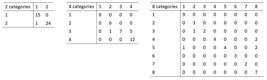
Confusion matrices for 2 (a = 0, b = 0 and k = 10), 4 (a = 0, b = 0 and k = 10) and 8 (a = 0, b = -1 and k = 10) categories.

Table 2:
Global variance (GV) for the 12 versions of the generalized multiquadric radial basis functions, for k = 10and k = 100 neighbors, in the spatial interpolation for 2, 4, and 8 categories in the validation set.

Scenarios	a	b	k = 100 (Global)	k = 10 (Local)
I (2 categories)	0	-1	0.375	0.480
	0	0	0.469	0.480
	0	1	0.439	0.480
	5	-1	0.469	0.480
	5	0	0.420	0.480
	5	1	0.420	0.480
	50	-1	0.399	0.480
	50	0	0.420	0.480
	50	1	0.420	0.480
	500	-1	0.420	0.480
	500	0	0.420	0.480
	500	1	0.420	0.480
II (4 categories)	0	-1	0.304	0.694
	0	0	0.656	0.708
	0	1	0.489	0.719
	5	-1	0.674	0.694
	5	0	0.489	0.708
	5	1	0.429	0.719
	50	-1	0.489	0.690
	50	0	0.401	0.708
	50	1	0.371	0.708
	500	-1	0.339	0.708
	500	0	0.339	0.694
	500	1	0.304	0.708
III (8 categories)	0	-1	0.489	0.821
	0	0	0.748	0.831
	0	1	0.489	0.830
	5	-1	0.800	0.831
	5	0	0.536	0.831
	5	1	0.489	0.831
	50	-1	0.489	0.824
	50	0	0.489	0.811
	50	1	0.489	0.820
	500	-1	0.489	0.811
	500	0	0.489	0.811
	500	1	0.489	0.820

Figure 6:
MapBiomas study area.

• DATA AVAILABILITY
  The datasets generated during and/or analyzed during the current study are available from the corresponding author on reasonable request.

• Edited by
  Silvana Philippi Camboim and Rodrigo Affonso de Albuquerque Nobrega.

Data availability

The datasets generated during and/or analyzed during the current study are available from the corresponding author on reasonable request.

Publication Dates

• Publication in this collection
  29 May 2026
• Date of issue
  2026

History

• Received
  13 Oct 2025
• Accepted
  07 Apr 2026