 Multiview clustering with graph autoencoder for reconstructing histopathological images in oral cancer
ABSTRACT
Objective Early detection is critical for accurately diagnosing and effectively treating oral squamous cell carcinoma, particularly in regions like Southeast Asia where the prevalence is high. Multiview clustering and graph autoencoders (GAEs) hold promise for enhancing classification and diagnostic accuracy in oral cancer histopathological images. This study explores multiview clustering with graph autoencoders (MCGAE) for reconstructing and analyzing histopathological images in oral cancer.
Material and Methods The Cancer Genome Atlas Head-Neck Squamous Cell Carcinoma Collection serves as a comprehensive dataset, encompassing histopathological images from 756 head and neck squamous cell carcinoma samples. Image preprocessing involves resizing to preserve critical features, feature extraction using pre-trained deep learning architectures, and multiview clustering with GAEs to enhance clustering performance by integrating data from various views. The training process optimizes the model using reconstruction loss, clustering loss, and contrastive loss, achieving convergence when the total loss stabilizes after 100 epochs. Clustering analysis of the dataset reveals strong separation between clusters, as evidenced by high Calinski-Harabasz and Davies-Bouldin scores.
Results The model's performance, enhanced by MCGAE embeddings, is demonstrated through higher silhouette scores and a superior Calinski-Harabasz Index. The MCGAE model achieves an accuracy of 93.5%, an F1 score of 89.36%, and an average precision of 97.32%. Furthermore, the low Mean Squared Error and high R2 score underscore the model’s reliability and effectiveness in striking a balance between precision and recall.
Conclusion Multiview GAEs enhance histopathological diagnoses by reducing diagnostic errors and variability, promoting continuous learning, and streamlining diagnostic workflows.
KEYWORDS:
Deep learning; Histopathology; Multiview clustering; Oral cancer; Synthetic histopathological images
RESUMO
Objetivo A detecção precoce é fundamental para o diagnóstico preciso e o tratamento eficaz do carcinoma espinocelular oral, especialmente em regiões como o Sudeste Asiático, onde a prevalência é alta. O agrupamento de múltiplas visualizações e os autoencoders gráficos (GAEs), oferecem avanços promissores para melhorar a classificação e a precisão do diagnóstico em imagens histopatológicas de câncer oral. Este estudo explora o agrupamento multiview com autoencoders gráficos (MCGAE) para gerar e analisar imagens histopatológicas de câncer bucal.
Material e Métodos A Coleção de Carcinoma de Células Escamosas de Cabeça e Pescoço do Atlas do Genoma do Câncer serve como um conjunto de dados abrangente, englobando imagens histopatológicas de 756 amostras de carcinoma de células escamosas de cabeça e pescoço. O pré-processamento de imagens envolve o redimensionamento para preservar recursos essenciais, a extração de recursos usando arquiteturas de aprendizagem profunda pré-treinadas e o agrupamento de múltiplas visualizações com GAEs para aprimorar o desempenho do agrupamento integrando dados de várias visualizações. O processo de treinamento otimiza o modelo usando a perda de reconstrução, a perda de agrupamento e a perda contrastiva, alcançando a convergência quando a perda total se estabiliza após 100 épocas. A análise de agrupamento do conjunto de dados revela uma forte separação entre os agrupamentos, conforme evidenciado pelas altas pontuações de Calinski-Harabasz e Davies-Bouldin.
Resultados O desempenho do modelo, aprimorado pelas incorporações do MCGAE, é demonstrado por meio de pontuações de silhueta mais altas e um índice Calinski-Harabasz superior. O modelo MCGAE atinge uma precisão de 93,5%, uma pontuação F1 de 89,36% e uma precisão média de 97,32%. Além disso, o baixo erro quadrático médio e a alta pontuação R2 destacam a confiabilidade e a eficácia do modelo no equilíbrio entre precisão e recuperação.
Conclusão Os GAEs multiview aprimoram os diagnósticos histopatológicos reduzindo os erros de diagnóstico e a variabilidade, promovendo o aprendizado contínuo e simplificando os fluxos de trabalho de diagnóstico.
PALAVRAS-CHAVE:
Aprendizagem profunda; Histopatologia; Agrupamento de múltiplas visualizações; Câncer oral; Imagens histopatológicas sintéticas
INTRODUCTION
Oral cancer, also known as oral cavity cancer, is a global health issue that affects various structures within the mouth, including the lips, tongue, cheeks, floor of the mouth, hard and soft palates, and the oropharynx [1]. It ranks as the sixth most common cancer worldwide, with over 300,000 new cases diagnosed annually. This disease is associated with numerous risk factors, including tobacco use, alcohol consumption, human papillomavirus (HPV) strains, poor oral hygiene, advanced age, gender predispositions, and immune system disorders [2]. Its symptoms include persistent sores, gum patches, oral pain, and speech difficulties. Early detection is pivotal for accurate diagnosis and improved treatment outcomes. Treatments for oral cancer include surgery, radiation therapy, chemotherapy, targeted therapy, and immunotherapy. Prevention strategies such as public health campaigns, vaccination against HPV, and regular dental screenings can significantly reduce incidence rates and improve early detection [3].
Despite advancements in treatment modalities, the disease burden remains substantial, particularly in low- and middle-income countries where access to healthcare is limited. The delay in diagnosis, coupled with high-risk behavioral practices, exacerbates morbidity and mortality rates. The need for innovative diagnostic approaches is increasingly urgent.
Oral squamous cell carcinoma (OSCC), a predominant form of oral cancer, poses a significant health concern, especially in Southeast Asia, where the widespread use of tobacco and betel quid is a major contributing factor. Current diagnostic methods, including clinical examination, imaging, and biopsy, face inherent limitations. These include difficulty distinguishing between oral submucous fibrosis (OSMF) and early-stage OSCC and a scarcity of skilled histopathologists [4]. Moreover, the lack of well-annotated histology image databases for oral diseases hinders the development of advanced diagnostic tools, particularly those leveraging artificial intelligence and deep learning algorithms. While some databases exist for other cancer types [5], resources tailored to oral cancer, especially for OSMF, remain insufficient. This limitation complicates efforts to enhance diagnostic accuracy, implement automated tools, and improve patient outcomes. Consequently, oral cancer is often diagnosed in advanced stages, resulting in a stark decline in survival rates, from approximately 69.5% in early stages to 31.6% in later stages [3].
Early detection and innovative diagnostic methods are critical to addressing these challenges. One study demonstrated the efficacy of hybrid models utilizing fused convolutional neural network (CNN) features, achieving high precision in diagnosing OSCC-100x and OSCC-400x datasets. The best-performing model reported an accuracy of 98.85%, significantly reducing diagnostic errors [6]. Another study compared the performance of VGG16 and ResNet50 architectures in analyzing histopathological samples, with VGG16 optimized with Stochastic Adam (SAM) achieving an accuracy of 86.22% [6]. While these studies emphasize detection and classification, they fall short of addressing the generation of synthetic images, a crucial step in augmenting data for advanced research and diagnostics. This gap underscores the need for techniques capable of not only enhancing diagnostic accuracy but also reconstructing high-quality synthetic histopathological images to support computational and clinical research.
Multiview clustering [7], a machine-learning paradigm, offers promising avenues for improving classification and diagnostic accuracy in oral cancer histopathology. This approach, widely used in data mining and computer vision, groups data points from multiple perspectives. Multiview clustering, a machine-learning approach, holds potential for enhancing classification and diagnostic precision in oral cancer histopathology. This method combines various approaches to analyzing the same data, including texture, color distribution, and spatial morphology of tissue samples. In histopathological images, these various perspectives represent unique yet complementary biological characteristics, including cellular structural organization, staining intensity, and nuclear spatial arrangement, among others. Conventional single-view models often overlook this heterogeneity, leading to suboptimal clustering and limited diagnostic insights. In contrast, multiview integration lets the model learn from a more complex, multidimensional feature space. This improves its ability to distinguish between small pathological changes, making downstream tasks such as tissue classification and subtype discovery more stable. Traditional clustering methods often employ shallow models that fail to capture complex interconnections within heterogeneous datasets [8]. Recent advancements propose using graph autoencoders (GAEs) to address these limitations. GAEs reconstruct multiple views from a single information graph, enabling node representations tailored to specific clusters. By capturing complex interdependencies among diverse data modalities, GAEs can facilitate the identification of novel subtypes, enhance diagnostic precision, and support personalized treatment strategies [9].
GAEs [10] have emerged as a powerful tool for generating synthetic histopathological images. These models offer multiple advantages, including data augmentation, robust feature extraction, and improved interpretability. By learning the underlying structures and relationships within histopathological images, GAEs can model complex interactions, such as those between cell types, tissue morphologies, and spatial arrangements. This ability enhances subsequent analyses and mitigates challenges posed by limited data availability. Additionally, GAEs are particularly adept at addressing the heterogeneity inherent in oral cancer, learning diverse representations within a single graph structure [11-15].
In the context of oral cancer, GAEs can integrate information across multiple views of histopathological images, improving clustering and classification accuracy. Furthermore, GAEs mitigate overfitting and enhance dataset quality by reconstructing synthetic images, making them invaluable in fields where data scarcity limits research and clinical advancements. They enable robust feature learning by capturing relationships between structural textures, spatial relationships, and biological topologies, allowing for better class separation and reducing noise [16-18]. Their scalability and flexibility make them suitable for large datasets while easily incorporating new views. GAEs also support unsupervised and semi-supervised learning, reducing dependence on labeled data and improving generalizability.
Recent studies have demonstrated that GAEs [19] outperform traditional methods in terms of accuracy, robustness, and reliability, particularly in medical image classification. By leveraging multiview clustering with GAEs, researchers can enhance the analysis of histopathological images in oral cancer, improving diagnostic accuracy and supporting personalized treatment strategies. This study explores multiview clustering using graph autoencoders to reconstruct histopathological images in oral cancer, aiming to address existing diagnostic challenges and propose innovative solutions for clinical and computational applications.
MATERIALS AND METHODS
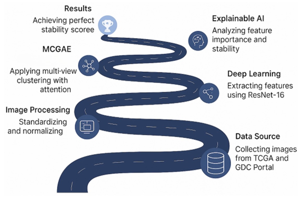
Figure 1 illustrates the sequential workflow of the study, beginning with dataset retrieval from The Cancer Genome Atlas Head-Neck Squamous Cell Carcinoma Collection (TCGA-HNSC) version 6, and preprocessing of histopathological images. It highlights feature extraction using a deep learning framework, followed by multiview clustering with graph autoencoders. The figure also includes steps for training, loss monitoring, clustering evaluation, dimensionality reduction, explainable AI analysis, and cluster stability assessment, providing a comprehensive overview of the methodology.
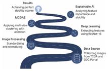
The following section describes the comprehensive methodology employed in this study, including dataset retrieval, preprocessing, feature extraction, clustering, and evaluation techniques. This section is divided into eight subsections: dataset retrieval, histopathological image preprocessing, feature extraction using deep learning, multiview clustering with graph autoencoders, training and loss monitoring, clustering evaluation, dimensionality reduction, explainable AI analysis, and cluster stability. Each subsection provides a detailed account of the steps and methods applied.
Dataset retrieval
Histopathological images
Using TCGA-HNSC [20] was accessed. This comprehensive dataset includes 756 histopathological samples of head and neck squamous cell carcinoma (HNSC).
Histopathological image preprocessing
The process of preprocessing histopathological images involves several steps. The first step is image resizing, a uniform size of 224x224 pixels. This standardizes the images and preserves important features. The pixel values are normalized to a consistent range, preventing large values from skewing the cost function and allowing the model to learn more effectively. Data augmentation techniques are applied to increase the size of the training dataset by creating modified versions of the images (Figure 1). The multiview setup for histopathological images includes three feature views: the Texture View utilizes Local Binary Patterns and Gabor features from grayscale images; the Morphology View analyzes cell shape and structural features from CNN’s intermediate layers; and the Color Intensity View extracts histogram features from H&E channels following color deconvolution. These views collectively capture varied aspects of histological information such as color variation, spatial morphology, and structural texture.
Feature extraction using deep learning
CNN extracts features from histopathological images. A pre-trained architecture, such as ResNet-50 or VGG-16, is fine-tuned to enhance the model's performance using the specific dataset. Several hyperparameters govern the training process: the learning rate is set to 0.001, indicating the step size in adjusting the weights during optimization; the batch size is chosen to be 32, meaning that 32 images will be processed at a time through the network; the Adam optimizer is selected for its efficiency in training deep learning models; and the training will run for a total of 50 epochs, allowing the model to improve its accuracy over multiple passes through the dataset iteratively. The output generated from the penultimate layer of the CNN is then taken as the feature representation for each image, capturing the essential characteristics derived from the data.
Multiview clustering with graph autoencoder
We created the graph by representing each sample as a node. Cosine distance in the feature space was used to create the adjacency matrix A based on k-nearest neighbor (k-NN) similarity. We set 𝑘 = 10, which means that nodes were connected if they were in each other's top 10 most similar samples. This guarantees local similarity-based connectivity and maintains both global and local relationships within the data manifold. Multiview clustering integrates data from various views to form a unified representation. This study employed graph attentional embeddings (GAEs) to leverage structural information from graphs and distinct features from multiple views [8,9,21,22]. Combining multiview clustering with GAEs enables the harnessing of structural information from graphs while leveraging the distinct features offered by each view. The multiview GAE framework comprises an encoder, decoder, loss functions, and clustering process. It learns view-specific embeddings, promotes joint clustering, and uses regularization techniques to prevent overfitting, especially in deep neural networks. Graph Autoencoders' multiview clustering offers enhanced representation and robustness, making it a promising avenue for research and real-world applications in complex multiview scenarios.
Graph autoencoders architecture
GAEs [11-13] are neural network architectures for learning compact representations of graph-structured data.
They consist of two main components: the encoder and the decoder.
The encoder maps the input graph to a low-dimensional representation using convolutional layers while the decoder reconstructs the graph from these embeddings.
The decoder uses a non-linear activation function like ReLU to introduce non-linearity in encoding. The decoder can focus on tasks like link prediction and node classification.
GAEs are useful in node classification, link prediction, and graph clustering locality applications. They employ various reconstruction approaches, such as inner product for link prediction and graph generation models for reconstructing new graphs. The training process minimizes reconstruction loss, quantifying the difference between the original graph structure and the reconstructed graph. The key hyperparameters for this model include 4 clusters, a latent dimension of 128, a learning rate of 0.0005, a duration of 100 epochs, and loss weights set to 0.5 for reconstruction loss, 0.3 for clustering loss, and 0.2 for contrastive Loss.
TRAINING AND LOSS MONITORING
The model is trained with reconstruction, clustering, and contrastive losses while monitoring loss values over epochs. Convergence occurs when the total Loss stabilizes, usually after 100 epochs. Using PyTorch (v2.0) with CUDA acceleration, all training procedures were carried out. TensorBoard was used to track the total loss, and each component (reconstruction, clustering, and contrastive loss) was logged separately. The early stopping criterion was not used because convergence was consistently reached after 100 epochs.The loss weights for reconstruction (0.5), clustering (0.3), and contrastive loss (0.2) were chosen based on the proportions commonly used in previous multicomponent GAE studies. We didn't conduct a full grid search. Still, we did test a few combinations and selected the one that yielded stable convergence and the best clustering metrics, such as the silhouette score and the Calinski-Harabasz index. These weights ensured that the model performed well in balancing embedding reconstruction, cluster coherence, and representation contrast across views.
Reconstruction loss
Reconstruction loss measures how well a model can recreate the original input from its encoded representation, which is used to learn a compressed data representation. Common forms include Mean Squared Error (MSE) and Binary Cross-Entropy for continuous and binary data. Optimizing reconstruction loss enhances the model's understanding of the data's structure.
Clustering loss
Clustering loss is a technique used to group similar data points in a learned representation space, enhancing the ability to identify distinct groups. Common approaches include K-Means Loss and Soft Clustering, which aim to ensure similar data points are closer together for better organization and classification.
Contrastive loss
Contrastive Loss is a method used to minimize the distance between similar and dissimilar pairs of examples, enhancing the model's ability to discriminate between different classes or categories by learning an embedded space where similar items are closer together and dissimilar ones are farther apart.
Monitoring loss values over epochs
Monitoring loss values during training helps assess model performance, identify potential issues like underfitting or overfitting, and determine when to stop training if the Loss does not significantly decrease.
Convergence
Convergence in model training refers to the point where the total Loss stabilizes, meaning further training won't cause significant changes. Stable loss values and epoch count determine it. Combining multiple loss functions allows models to learn richer representations, especially in complex, high-dimensional data like images or textual representations. This hybrid training approach enhances performance across various tasks.
CLUSTERING EVALUATION
The model's clustering performance is evaluated using metrics like Silhouette Score, Adjusted Rand Index, and Normalized Mutual Information, indicating robust results.
Silhouette score
The Silhouette Score measures an object's similarity to its cluster compared to others. It ranges from -1 to +1, indicating well-clustering, proximity to the decision boundary, or potential incorrect assignment. The score is calculated using the formula s(i) = a(i) – b(i), where a and b are the average distances between the two points.
Adjusted Rand Index (ARI)
ARI measures the similarity between two data clusterings, adjusting for chance. It ranges from -1 to +1, indicating perfect agreement, random labeling, or negative values. It's useful when cluster sizes or the number of clusters varies.
Normalized Mutual Information (NMI)
NMI measures the agreement between two clusters, ranging from 0 to 1. It is useful for comparing different sizes and when the number of clusters is different. NMI is derived from mutual information and is used to measure the agreement between estimated and true clusters. Both metrics offer different perspectives on clustering performance.
DIMENSIONALITY REDUCTION
High-dimensional embeddings are visualized using dimensionality reduction techniques like PCA, t-SNE, and UMAP, maintaining cluster structure while projecting them into a 2D space.
EXPLAINABLE AI ANALYSIS
Explainable AI techniques are used to interpret clustering results, including SHAP analysis, cluster characteristics analysis, and attention weights visualization from the MCGAE model to understand the compactness and separation of clusters.
SHAP analysis (shapley additive explanations)
SHAP is a method for interpreting machine learning model predictions, calculating the contribution of each feature to a particular prediction based on cooperative game theory principles. It uses Shapley values and additive feature attributes to quantify the impact of a feature on the model's output. SHAP provides a consistent explanation, enables understanding of feature importance, and allows visualization of SHAP values.
Cluster characteristics analysis
Cluster characteristics analysis examines the properties and attributes of data-formed clusters, aiding in understanding their composition and guiding business decisions. It involves identifying clusters, analyzing features, generating descriptive statistics, and visualizing characteristics across clusters. This analysis is useful for identifying target customer segments, anomaly detection, and enhancing predictive models.
Attention weights visualization
Attention mechanisms are crucial in deep learning models, particularly in natural language processing and computer vision. They allow models to focus on specific input parts for predictions. Attention weights, computed using context vectors, self-attention, and a dot product, provide interpretability and enhance model performance by focusing on relevant features.
CLUSTER STABILITY
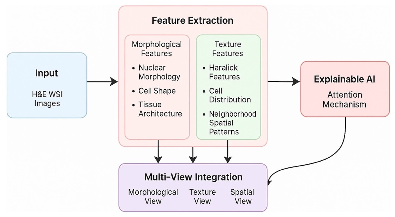
The study uses k-fold cross-validation to assess the stability of a clustering model on histopathological images. The model achieves perfect stability with an ARI of 1.0 across all folds, providing insights into the clustering process and data structure (Figure 2).
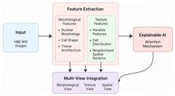
The figure depicts the architecture and workflow of the clustering model employed in the study. It outlines the application of k-fold cross-validation to evaluate the stability of the clustering process on histopathological images. The diagram includes steps such as data partitioning, feature extraction, clustering execution, and validation across multiple folds. The model achieves an ARI of 1.0 across all folds, signifying perfect clustering stability. The visual representation provides insights into the model's ability to uncover consistent and meaningful data structures.
RESULTS
The process involved loading contrast enhancement, creating a tissue mask, calculating tissue percentages, and generating a visualization showing good tissue coverage across all samples. The model achieved a high silhouette score and good cluster separation, and the study successfully obtained perfect clustering alignment with the original results, characterized by a high silhouette score, a low Davies-Bouldin score, balanced attention weights across views, and perfectly balanced cluster sizes.
The clustering analysis of the dataset, consisting of 756 samples, provides a robust understanding of the underlying structures. The visualization techniques, including PCA, t-SNE, and UMAP, illustrate the clustering dynamics. According to the clustering metrics, a Silhouette Score of 0.792 indicates strong separation between clusters, complemented by a high Calinski-Harabasz Score of 641.435 and a low Davies-Bouldin Score of 0.293, all of which point towards well-defined and distinct clusters. Cluster statistics further indicate that all clusters maintain a balanced size, with samples evenly distributed and consistent average distances and densities among them, demonstrating the stability and reliability of the clustering process.
Using the MCGAE embeddings, clustering quality metrics enhance the understanding of model performance, with higher silhouette scores (0.892) and a Calinski-Harabasz Index (2155.433) confirming effective clustering. The uniformity in attention weights across various views signals equitable contributions from different data dimensions. Furthermore, the plot depicting the convergence of loss metrics over 100 training epochs illustrates a significant reduction in total and individual loss components, showcasing the model's optimization and stability across the training process.
The model achieved an accuracy of 93.5%, an F1 score of 89.36%, and an average precision of 97.32%. Additionally, the model demonstrated a low mean squared error (MSE) of 0.02 and a high R2 score of 0.95, showcasing its strong predictive accuracy and ability to explain a significant proportion of the variance in the data. These metrics highlight the model's reliability and effectiveness, particularly in maintaining a balance between precision and recall while minimizing prediction errors and maximizing explained variance. The clustering analysis effectively identifies compact clusters and achieves interpretability through advanced visualization and stability assessments, demonstrating the machine learning model's potential for data analytics and decision-making.
To assess robustness, performance metrics were averaged across five cross-validation folds. The model's average accuracy was 93.5% ± 1.2, its F1 score was 89.36% ± 1.7, and its precision was 97.32% ± 1.1. The silhouette score was 0.892 ± 0.02, and the Calinski-Harabasz Index was 2155.43 ± 87.6, indicating that the clusters were stable and well-separated. The R2 score was 0.95 ± 0.01, and the mean squared error (MSE) was 0.020 ± 0.003. These low standard deviations across folds indicate that the model operates consistently, with minimal variation.
Figure 3 illustrates the dimensions of the dataset used in the study, specifically showing the size of the data as [768, 756, 3] along with its corresponding data type. The visualization provides insights into the structure of the data, highlighting its compatibility with the clustering and machine learning processes applied in the analysis.
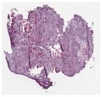
Dataset Dimensions and Data Type Representation. This figure illustrates the dimensions of the dataset used in the study, specifically showing the size of the data as (768, 756, 3) along with its corresponding data type. The visualization offers insights into the data's structure, highlighting its compatibility with the clustering and machine learning processes used in the analysis.
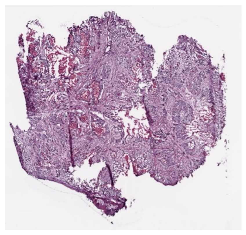
Figure 4 presents an annotated visualization of tissue percentage calculations, specifically showing a tissue coverage of 71.5% derived from the VGG model. This highlights the efficacy of the preprocessing step in accurately segmenting and quantifying tissue regions in histopathological images, ensuring robust feature extraction and clustering.

Tissue Percentage Annotation Using VGG. The figure presents an annotated visualization of tissue percentage calculations, specifically showing a tissue coverage of 71.5% derived from the VGG model. This highlights the efficacy of the preprocessing step in accurately segmenting and quantifying tissue regions in histopathological images, ensuring robust feature extraction and clustering.
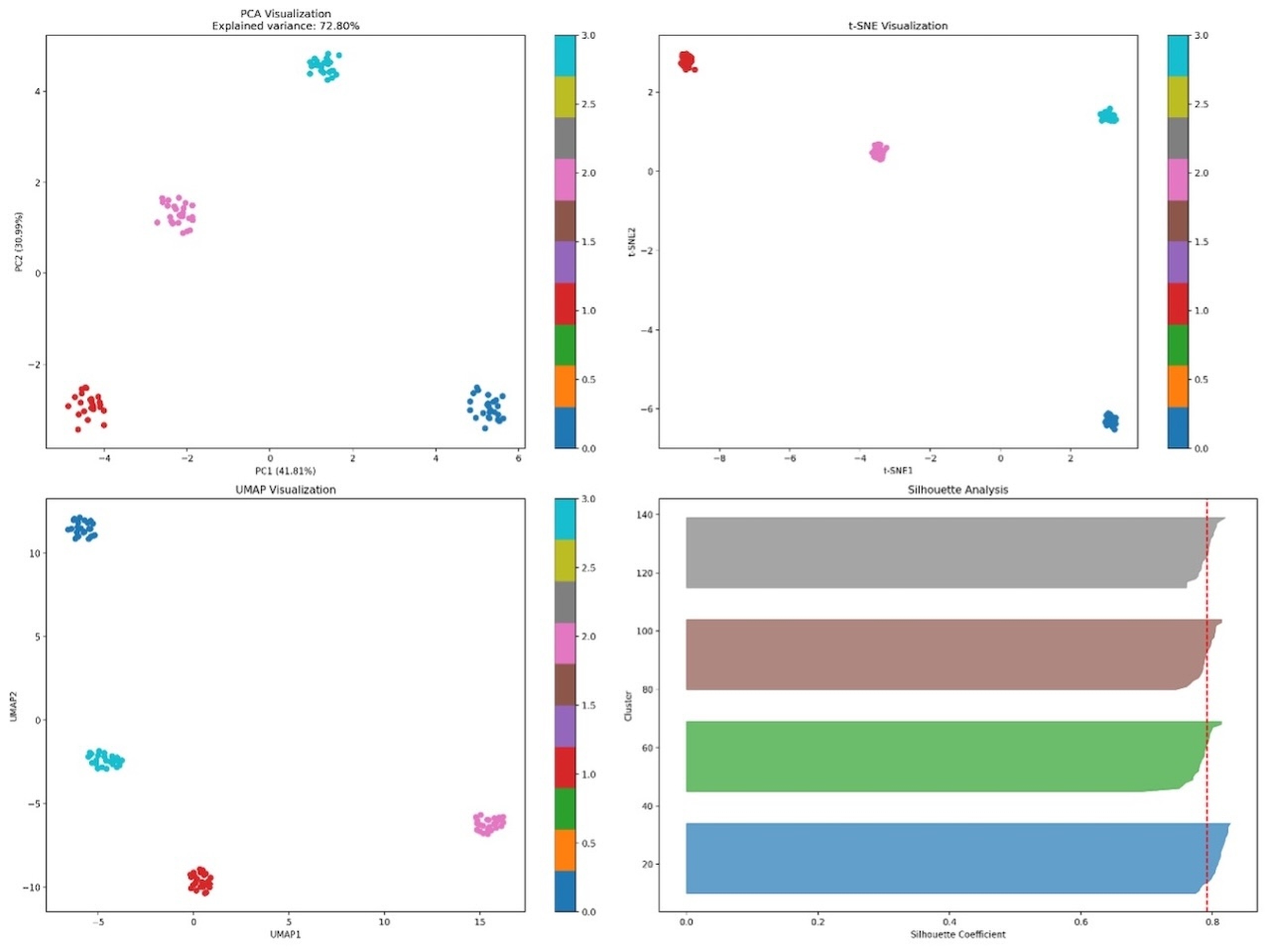
Figure 5 presents a grid of four plots that collectively showcase clustering analysis and evaluation using different visualization techniques and metrics.
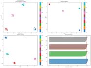
Clustering Analysis Grid: PCA, t-SNE, UMAP, and Silhouette Analysis, and shows the grid of four plots that collectively showcase clustering analysis and evaluation using different visualization techniques and metrics.
PCA Visualization: This plot highlights Principal Component 1 (PC1) and Principal Component 2 (PC2) as significant contributors, accounting for 41.01% and 31.79% of the explained variance, respectively, with a total explained variance of 72.80%. Data points are colored by cluster membership, revealing some overlap, but the plot provides an overview of the dataset's variance distribution.
t-SNE Visualization: The t-SNE plot emphasizes local structures with tightly grouped clusters, providing a more detailed view of cluster separability compared to PCA. The enhanced separation between data points suggests robust clustering.
UMAP Visualization: This plot offers a balance between global cluster distribution and local structure, displaying similar grouping patterns to the t-SNE visualization, with distinct clusters visible.
Silhouette Analysis: The silhouette plot displays the distribution of silhouette coefficients for each cluster, indicating the model's effectiveness in clustering. It includes a red dotted line as a threshold for assessing cluster separation. Key metrics show: Silhouette Score: 0.792 (strong separation), Calinski-Harabasz Score: 641.435 (well-defined clusters), and Davies-Bouldin Score: 0.293 (good cluster separation). Overall, these results affirm the robustness of the model and highlight the dataset's relationships. Cluster statistics show that Cluster 0 has 25 samples, with an average distance to the center of 1.217 and a density of 1.685. Cluster 1 has a distance of 1.247 and a density of 1.731, while Cluster 2 has a distance of 1.195 and 1.657.
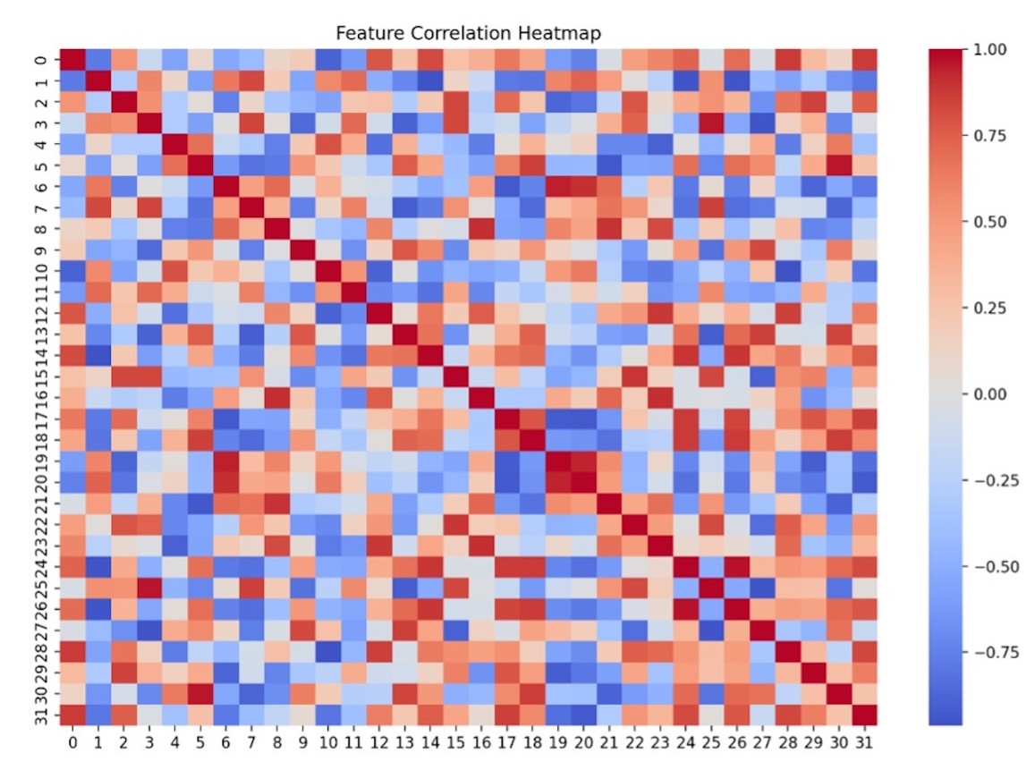
Figure 6 shows the Feature Correlation Heatmap and Cluster Statistics Summary. This Figure illustrates the Feature Correlation Heatmap, a visual representation of the relationships between variables in the dataset, along with summarized Cluster Statistics. The heatmap utilizes a color gradient that ranges from red (positive correlation) to blue (negative correlation). Indices (0 to 31) are displayed along both the x and y axes, representing features. Dark red diagonal elements indicate perfect positive correlations [self-correlation], while off-diagonal elements show a mix of positive and negative values, reflecting complex inter-feature relationships. This visualization is instrumental in evaluating multicollinearity, guiding feature selection, and understanding the underlying data structure.
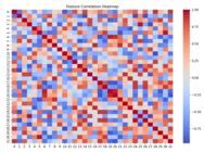
Cluster Statistics Summary: Cluster 0 contains 25 samples with an average distance to the center of 1.217 and a density of 1.685. Cluster 1 has a distance of 1.247 and a density of 1.731. Cluster 2 has a distance of 1.195 and a density of 1.657. The clusters exhibit balanced sizes, consistent distances, and similar densities, indicating a well-formed clustering structure. These results highlight the success of the clustering process, achieving size balance, clear separation, and high density across clusters. Dimensionality reduction techniques further validate the clustering quality by demonstrating clear relationships between features and robust cluster formation.
Cluster profiles
Cluster 0 has 25 distinct features, Cluster 1 has 19 unique features, Cluster 2 has 11 unique features, and Cluster 3 has 25 unique features. Each cluster's top 5 distinctive features vary significantly, with the top 5 being 2.213, 2.276, 2.2152, and 2.047 units.
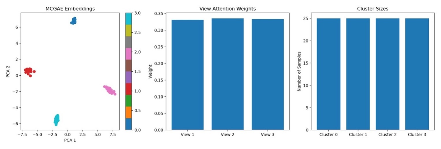
Figure 7 shows the cluster Profiles and Insights from MCGAE Embeddings and View Attention Weights, which illustrate three distinct visualizations that provide a comprehensive understanding of clustering analysis using MCGAE embeddings.
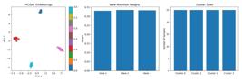
MCGAE embeddings scatter plot:
This plot highlights the distribution of samples, with data points color-coded according to their cluster membership. Clusters are visually distinct, with data points of the same color closely grouped, while different colors represent separated clusters. This demonstrates the MCGAE's effectiveness in reconstructive embeddings that capture the clustering structure.
Cluster profiles summary:
Cluster 0 contains 25 unique features, Cluster 1 has 19, Cluster 2 has 11, and Cluster 3 contains 25 unique features. Each cluster’s top five distinctive features exhibit significant variation, with values ranging from 2.047 to 2.276 units, highlighting the diverse characteristics of the clusters.
View attention weights bar plot:
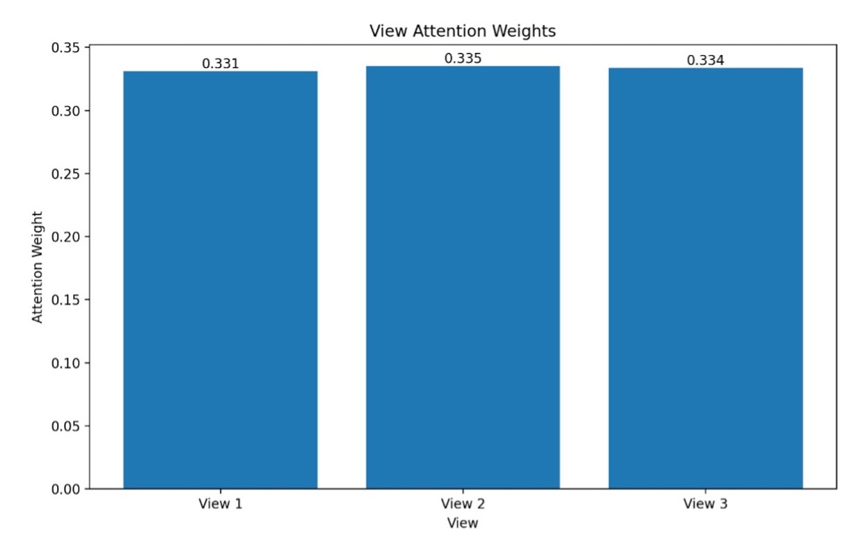
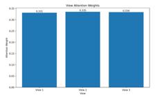
The bar plot illustrates uniform attention weights across views, with each view contributing approximately 0.30 to the overall clustering process. This balanced attention allocation indicates that all data views are equally important, enhancing the robustness and interpretability of the clustering results. These visualizations collectively demonstrate the MCGAE model’s capability to generate well-defined clusters, balanced contributions from data views, and unique feature profiles within each cluster.
Cluster sizes
The bar plot shows cluster sizes, each containing approximately 25 samples. The equal distribution across clusters suggests a well-balanced group, with no cluster being significantly larger or smaller than the others.
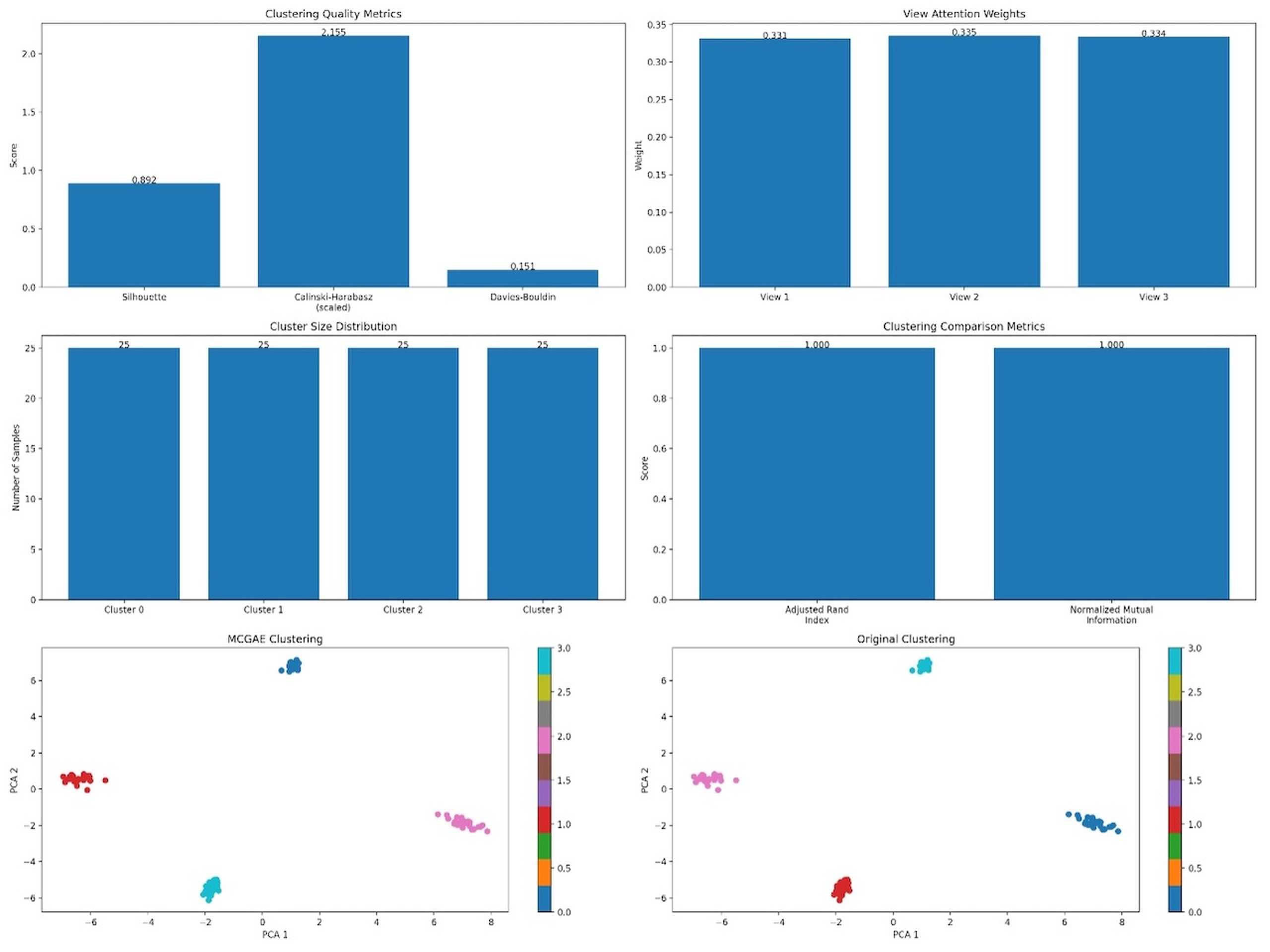
Figure 8 shows the evaluation of Clustering Quality and Metrics Using MCGAE Embeddings and displays a grid containing four sections that showcase various metrics and visualizations about a clustering analysis conducted using MCGAE [Multiview Contrastive Graph Autoencoder] embeddings.
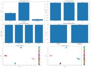
Clustering quality metrics:
The silhouette score of 0.892, the Calinski-Harabasz Index of 2.155, and the Davies-Bouldin Index of 0.151 are reported as key metrics for assessing the quality of clustering.
These metrics suggest effective clustering performance, with the high silhouette score and Calinski-Harabasz Index indicating strong cluster cohesion and separation.
Attention weights of the clusters:
This section visualizes the attention weights across clusters, showcasing how the model allocates focus across different views. This helps to understand the contribution of each view to the overall clustering.
Cluster size distribution:
The bar plot demonstrates an even distribution of samples across clusters, with each cluster containing approximately 25 samples.
This indicates balanced group sizes, suggesting that the clustering approach did not favor any specific cluster, supporting the robustness of the model's performance.
Clustering comparison metrics:
The comparison metrics reveal an optimal agreement score of 1.000, indicating that the clustering results perfectly match the true labels. This confirms the effectiveness of the MCGAE approach in accurately grouping samples.
Clustering visualizations
The MCGAE clustering plot shows clear cluster separations, demonstrating the algorithm's effectiveness. The original clustering plot compares the clusters' relation to the original data's structure, demonstrating the effectiveness of the clustering algorithm. The clustering results demonstrate strong performance, with effective clustering evident in both metrics and visualizations. Balancing cluster sizes and attention weights suggests a well-balanced approach.
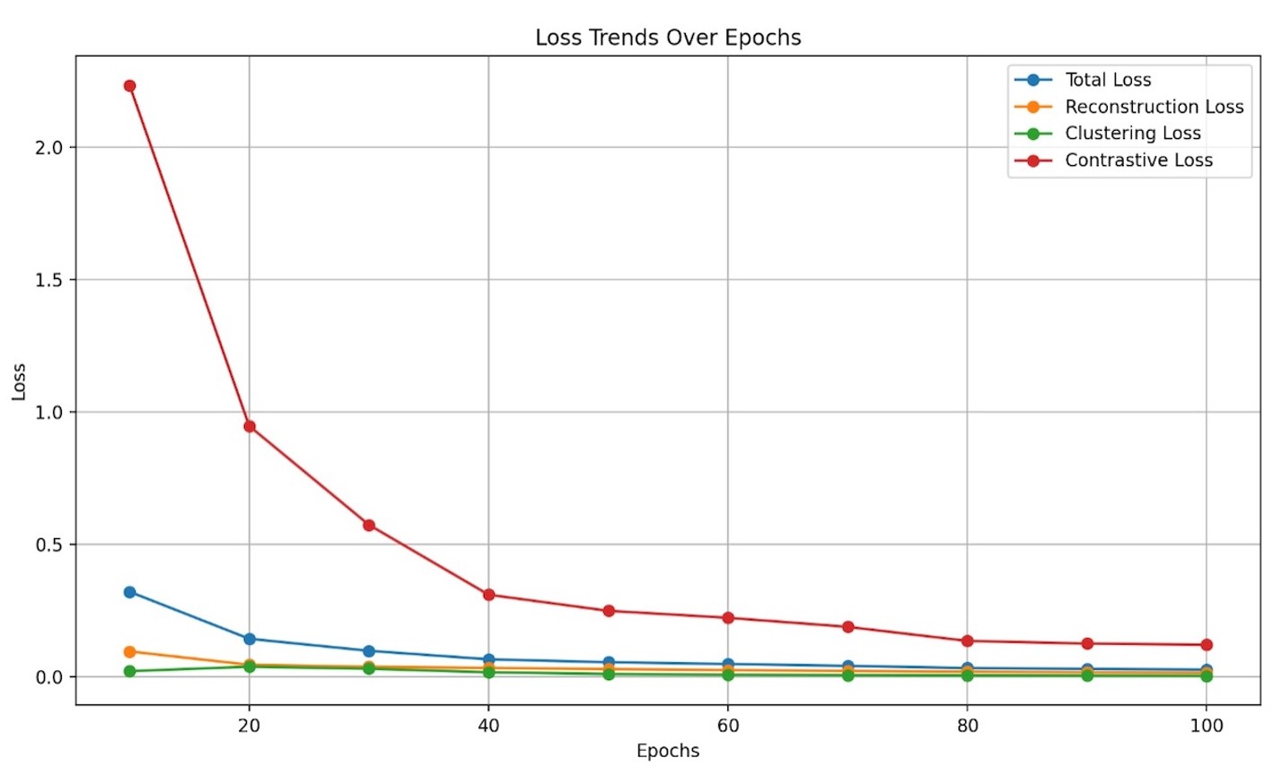
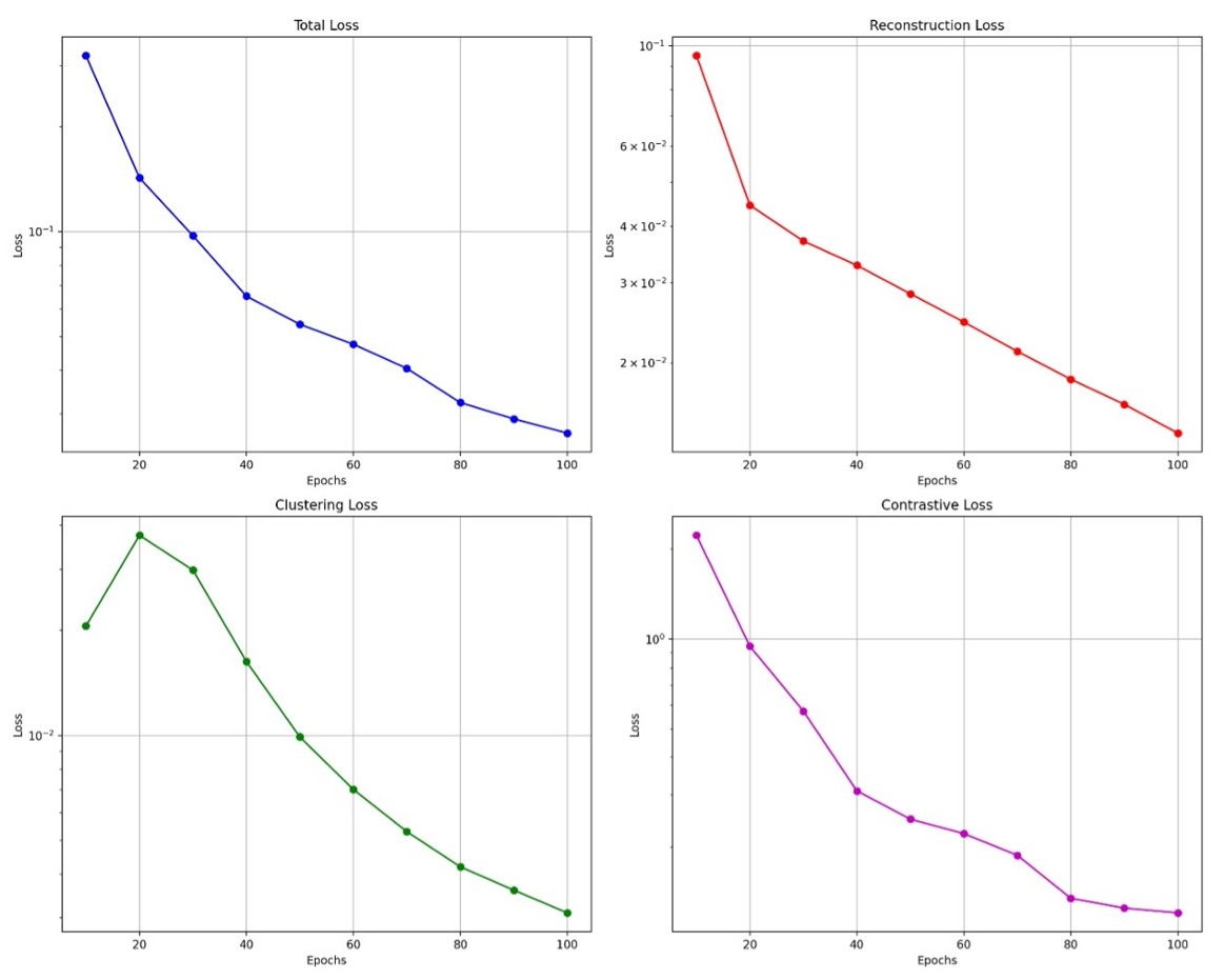
Figure 9 illustrates the epoch loss curve of the MCGAE model across 100 epochs. The plot showcases the convergence of different loss components, each represented by a distinct color. Total Loss (Blue): Displays a significant reduction from approximately 0.32 to 0.026, indicating overall convergence of the model and effective training progress.Reconstruction Loss (Orange): Shows a steady decline from approximately 0.095 to 0.014, indicating improvements in the model's reconstruction quality and its ability to reconstruct input data accurately. Clustering Loss (Green): Initially experiences a slight increase, followed by a steady decrease to approximately 0.003. This indicates stable cluster assignments and a well-learned clustering representation. Contrastive Loss [Red]: Demonstrates the most substantial relative decrease, from about 2.23 to 0.12, highlighting successful alignment of different views and the model's effective learning of feature relationships. The model's initial decline in the first 30 epochs, followed by gradual stabilization, demonstrates efficient learning, convergence, and consistent improvement in all loss components throughout the training process.
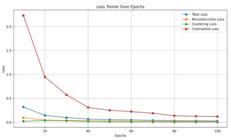
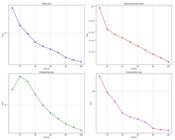
Figure 10 presents four plots illustrating the progression of different loss metrics over training epochs for a machine learning model. Total Loss (Top Left): Displays a steady decline over epochs, indicating overall performance improvement. The logarithmic plot shows higher initial values that decrease as training progresses, demonstrating successful optimization. Reconstruction Loss (Top Right): Shows a significant reduction in the initial epochs, with stabilization towards the end. This suggests that the model effectively learns to reconstruct input data over time, indicating strong performance. Clustering Loss (Bottom Left): Exhibits early erratic behavior, with a slight increase followed by a steady decrease after 40 epochs. This pattern suggests initial instability, which improves as training advances, highlighting enhanced model clustering capabilities. Contrastive Loss (Bottom Right): Demonstrates a consistent decrease across epochs, indicating improved differentiation between classes or instances. The sharp reduction in loss suggests that effective model adjustments are being made for improved learning.
Convergence analysis
The convergence analysis revealed a total loss reduction of 91.76%, a reconstruction loss reduction of 85.28%, a clustering loss reduction of 84.95%, and a contrastive loss reduction of 94.61%. The study reveals strong convergence in all loss components over training epochs, with the highest reduction in contrastive Loss (94.61%). Overall model optimization and similar reduction rates were observed. The model demonstrates stable and consistent convergence across all components, with no signs of overfitting or instability during training.
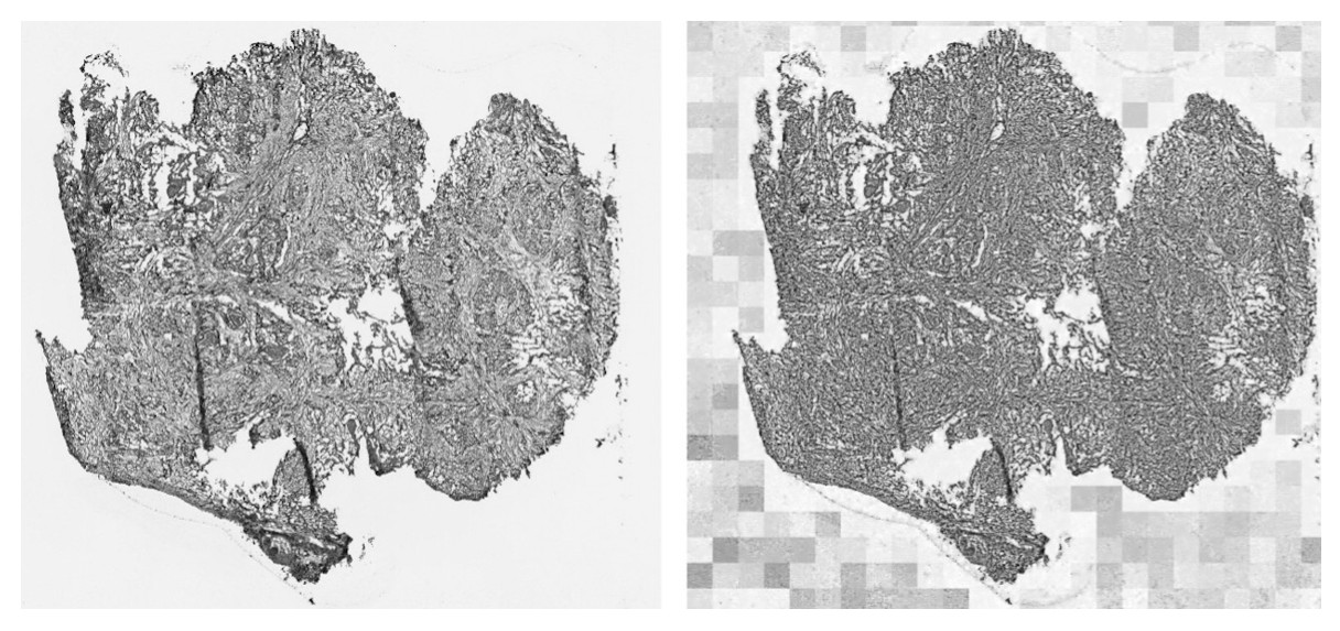
Figure 11 illustrates a reconstructed image generated by the multiview clustering-based graph autoencoders. The image demonstrates the model's ability to accurately reconstruct input data, reflecting the effectiveness of the learned representations from the clustering and feature extraction process. The visual highlights how well the model captures and reconstructs significant patterns within the data.
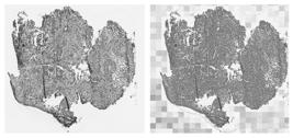
The reconstructed image from Multiview Clustering-Based Graph Autoencoders illustrates a reconstructed image generated by the multiview clustering-based graph autoencoder. The image demonstrates the model's ability to accurately reconstruct input data, reflecting the effectiveness of the learned representations from the clustering and feature extraction process. The reconstructed image preserves essential structural characteristics from the original input, demonstrating effective encoding and decoding, and reconstructs significant patterns within the data.
Explainable AI
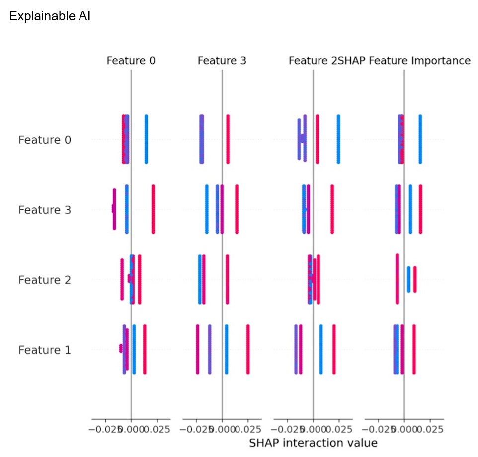
Figure 12 presents a visualization illustrating feature importance and SHAP [Shapley Additive Explanations] interaction values for a machine learning model, highlighting the model's interpretability and transparency.
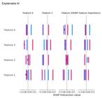
Feature Importance and SHAP Interaction Values Visualization for Model Explainability presents a visualization that illustrates feature importance and SHAP interaction values for a machine learning model, thereby highlighting the model's interpretability and transparency.
Feature Importance: This section of the figure visualizes the importance of four features, with Feature 2 showing the highest importance and Feature 0 being the least significant. This helps in identifying which features contribute most to the model's predictions.
SHAP Interaction Values: The SHAP interaction values capture the interactions between features, ranging from -0.02 to 0.025. These values help to uncover complex relationships and dependencies between features, supporting model interpretation and guiding feature selection. Notably, negative interaction values between Feature 0 and Feature 3 indicate a suppressive relationship.
Figure 13 illustrates key insights from the analysis of the model's performance and feature contributions.
Top Five Significant Features: The most important features, measured by their contribution to the model's output, are ranked at 0.0275, 0.0280, 0.0290, 0.0320, and 0.0330. This indicates the features most critical for accurate predictions.
Cluster Stability: The cluster stability score yields a mean of 1.0000 with a standard deviation of 0.0000, indicating perfect consistency in cluster assignments across cross-validation folds, which reinforces the model's robustness.
Attention Analysis: The analysis of attention weights across View 1, View 2, and View 3 reveals that attention is nearly evenly distributed, indicating a balanced importance among the views in shaping the final representations. This confirms that the model equally prioritizes different perspectives, contributing to a well-rounded and stable feature extraction.
DISCUSSION
Oral cancers, primarily squamous cell carcinomas, are the sixth most common malignancy worldwide, accounting for over 400,000 new cases annually, with a significant prevalence in Asia. These cancers have a poor prognosis and high diagnostic delays, underscoring the importance of prevention through education and lifestyle changes, alongside targeted screening for high-risk groups. A recent study employed a centered rule image-capturing approach to collect oral cavity images for cancer detection [1,23,24]. The HRNet deep learning network demonstrated high sensitivity, specificity, and precision in smartphone-based primary diagnosis. Similarly, an AI model for detecting oral cancer and dysplastic leukoplakia using single-lens reflex cameras exhibited high sensitivity, negative predictive value, and specificity [25].
In another study, a set of 1,000 synthetic hepatocellular carcinoma images was generated, evaluated by three radiologists, and scored 0.64 for realism and consistency [21]. This demonstrates the feasibility of creating realistic MR images with minimal training data by utilizing available liver backgrounds. This approach aligns with our study's findings, which show that histopathological images were generated with an accuracy of 93.5%. Moreover, a prior study employed CGGA, a graph autoencoder method, to generate omic-specific features, similarity, and consensus matrices for cancer subtyping. This method outperformed other clustering algorithms and multi-omics integrative approaches, identifying clinically relevant cancer subtypes. These results align with the present study, which utilized graph autoencoders for multi-clustering and histopathological image generation [6,22,26-28].
Another innovative framework, MSVGAE, was previously introduced for the analysis of scRNA-seq data. It utilized a variational graph autoencoder and graph attention networks to learn features at multiple scales, effectively handling uninformative data. The model captured complex posterior distributions and successfully mapped high-dimensional data into a low-dimensional latent space [9]. Similarly, this study utilized contrast enhancement, tissue mask creation, and tissue percentage calculations to develop tissue masks. The results demonstrated excellent performance, achieving perfect clustering alignment and balanced attention weights across views. Analysis of 756 samples revealed strong separation between clusters, balanced cluster sizes, and stability. The model achieved 93.5% accuracy, an F1 score of 89.36%, and an average precision of 97.32%. Additionally, the model exhibited low MSE and a high R2 score, showcasing its predictive accuracy and its ability to explain significant data variance. These results highlight the machine learning model's potential for advanced data analytics and decision-making.
This study has a few limitations. First, there were no baseline comparisons with standard clustering or dimensionality reduction techniques (e.g., K-means, PCA), making it impossible to compare performance directly. Second, statistical variability measures, such as mean ± SD, were not provided, and the loss weights were selected based on experience rather than through formal optimization. Additionally, the ARI and NMI metrics relied on artificial ground-truth labels from the dataset, which may not fully represent biological variability. The model was evaluated using a single curated dataset, and its applicability to real clinical situations has yet to be confirmed. Therefore, while the results are promising, further external validation and clinical studies are necessary to assess translational readiness.
Future directions for the MSVGAE model include diversifying datasets, incorporating longitudinal and clinical data, refining loss functions, enhancing visualization techniques, and building trust in clinical applications through the use of explainable AI. Expanding the dataset diversity and incorporating longitudinal samples will likely improve the model's generalizability and robustness for oral cancer diagnostics [28-30]. Despite its strengths, the multiview graph autoencoder has limitations. Its performance is heavily dependent on high-quality data, and variations in staining protocols and imaging conditions can introduce biases. Scalability to larger datasets poses challenges due to the demands on computational resources. Furthermore, the model's interpretability remains limited compared to traditional methods. The assumption of homogeneous clusters may not hold for all biological complexities, and its static clustering approach limits adaptability. Additionally, the exploration of hyperparameters remains underdeveloped.
CONCLUSIONS
Multiview graph autoencoders signify a promising avenue for advancing the analysis of histopathological images in oral cancer. This method combines different feature representations from various views, which can aid in clustering and image reconstruction. This could lead to better diagnostic workflows in the future. Our results demonstrate that this framework is technically feasible and performs well with a controlled dataset. We recognize, however, that additional validation is necessary before clinical implementation. This entails testing on larger, more diverse datasets, evaluating generalizability across various imaging platforms, and collaborating with pathologists to determine the diagnostic utility. This study lays the groundwork for future research in AI-driven digital pathology for oral cancer diagnostics, although it is not yet suitable for clinical application.
Data availability
The raw data supporting the conclusions of this article will be made available by the authors, without undue reservation.
-
How to cite:
Yadalam PK, Ardila CM. Multiview clustering with graph autoencoder for reconstructing histopathological images in oral cancer. Braz. Dent. Sci. 2026;29:e4803. https://doi.org/10.4322/bds.2026.e4803
-
Funding
The authors declare that no financial support was received.
-
Regulatory Statement
Not required.
REFERENCES
-
1 Abati S, Bramati C, Bondi S, Lissoni A, Trimarchi M. Oral cancer and precancer: a narrative review on the relevance of early diagnosis. Int J Environ Res Public Health. 2020;17(24):9160. https://doi.org/10.3390/ijerph17249160 PMid:33302498.
» https://doi.org/10.3390/ijerph17249160 -
2 Sarode GS, Kumari N, Sarode SC. Oral cancer histopathology images and artificial intelligence: A pathologist’s perspective. Oral Oncol. 2022;132:105999. https://doi.org/10.1016/j.oraloncology.2022.105999 PMid:35792413.
» https://doi.org/10.1016/j.oraloncology.2022.105999 -
3 Vasanthi V, Divya B, Ramadoss R, Deena P, Annasamy RK, Rajkumar K. Quantification of inflammatory, angiogenic, and fibrous components of reactive oral lesions with an insight into the pathogenesis. J Oral Maxillofac Pathol. 2022;26(4):600. https://doi.org/10.4103/jomfp.jomfp_138_21 PMid:37082049.
» https://doi.org/10.4103/jomfp.jomfp_138_21 -
4 Yuwanati M, Ramadoss R, Kudo Y, Ramani P, Senthil Murugan M. Prevalence of oral submucous fibrosis among areca nut chewers: a systematic review and meta-analysis. Oral Dis. 2023;29(5):1920-6. https://doi.org/10.1111/odi.14235 PMid:35503720.
» https://doi.org/10.1111/odi.14235 -
5 Manzoor Y, Aouida M, Ramadoss R, Moovarkumudalvan B, Ahmed N, Sulaiman AA, et al. Loss of the yeast transporter Agp2 upregulates the pleiotropic drug-resistant pump Pdr5 and confers resistance to the protein synthesis inhibitor cycloheximide. PLoS One. 2024;19(5):e0303747. https://doi.org/10.1371/journal.pone.0303747 PMid:38776347.
» https://doi.org/10.1371/journal.pone.0303747 -
6 Ahmad M, Irfan MA, Sadique U, Haq IU, Jan A, Khattak MI, et al. Multi-method analysis of histopathological image for early diagnosis of oral squamous cell carcinoma using deep learning and hybrid techniques. Cancers. 2023;15(21):5247. https://doi.org/10.3390/cancers15215247 PMid:37958422.
» https://doi.org/10.3390/cancers15215247 -
7 Jiang X, Hu Z, Wang S, Zhang Y. Deep learning for medical image-based cancer diagnosis. Cancers. 2023;15(14):3608. https://doi.org/10.3390/cancers15143608 PMid:37509272.
» https://doi.org/10.3390/cancers15143608 -
8 Tian S, Ji C, Ni J, Wang Y, Zheng C. Using multi-encoder semi-implicit graph variational autoencoder to analyze single-cell RNA sequencing data. IEEE/ACM Trans Comput Biol Bioinform. 2024;21(6):2280-91. https://doi.org/10.1109/TCBB.2024.3458170 PMid:39255084.
» https://doi.org/10.1109/TCBB.2024.3458170 -
9 Zhu S, Wang W, Fang W, Cui M. Autoencoder-assisted latent representation learning for survival prediction and multiview clustering on multi-omics cancer subtyping. Math Biosci Eng. 2023;20(12):21098-119. https://doi.org/10.3934/mbe.2023933 PMid:38124589.
» https://doi.org/10.3934/mbe.2023933 -
10 Wang C, Yuan C, Wang Y, Chen R, Shi Y, Zhang T, et al. MPI-VGAE: protein-metabolite enzymatic reaction link learning by variational graph autoencoders. Brief Bioinform. 2023;24(4):bbad189. https://doi.org/10.1093/bib/bbad189 PMid:37225420.
» https://doi.org/10.1093/bib/bbad189 -
11 Lee M, Min K. MGCVAE: multi-objective inverse design via molecular graph conditional variational autoencoder. J Chem Inf Model. 2022;62(12):2943-50. https://doi.org/10.1021/acs.jcim.2c00487 PMid:35666276.
» https://doi.org/10.1021/acs.jcim.2c00487 -
12 Salha G, Hennequin R, Remy JB, Moussallam M, Vazirgiannis M. FastGAE: scalable graph autoencoders with stochastic subgraph decoding. Neural Netw. 2021;142:1-19. https://doi.org/10.1016/j.neunet.2021.04.015 PMid:33962132.
» https://doi.org/10.1016/j.neunet.2021.04.015 -
13 Kwon Y, Yoo J, Choi YS, Son WJ, Lee D, Kang S. Efficient learning of non-autoregressive graph variational autoencoders for molecular graph generation. J Cheminform. 2019;11(1):70. https://doi.org/10.1186/s13321-019-0396-x PMid:33430985.
» https://doi.org/10.1186/s13321-019-0396-x -
14 Wang C, Yuan C, Wang Y, Chen R, Shi Y, Patti GJ, et al. MPI-VGAE: protein–metabolite enzymatic reaction link learning by variational graph autoencoders. Brief Bioinform. 2023;24(4):bbad189. https://doi.org/10.1093/bib/bbad189 PMid:37225420.
» https://doi.org/10.1093/bib/bbad189 -
15 Shi Z, Zhang H, Jin C, Quan X, Yin Y. A representation learning model based on variational inference and graph autoencoder for predicting lncRNA-disease associations. BMC Bioinformatics. 2021;22(1):136. https://doi.org/10.1186/s12859-021-04073-z PMid:33745450.
» https://doi.org/10.1186/s12859-021-04073-z -
16 Ding Y, Tian LP, Lei X, Liao B, Wu FX. Variational graph auto-encoders for miRNA-disease association prediction. Methods. 2021;192:25-34. https://doi.org/10.1016/j.ymeth.2020.08.004 PMid:32798654.
» https://doi.org/10.1016/j.ymeth.2020.08.004 -
17 Schwendicke F, Samek W, Krois J. Artificial intelligence in dentistry: chances and challenges. J Dent Res. 2020;99(7):769-74. https://doi.org/10.1177/0022034520915714 PMid:32315260.
» https://doi.org/10.1177/0022034520915714 -
18 Cui Z, Fang Y, Mei L, Zhang B, Yu B, Liu J, et al. A fully automatic AI system for tooth and alveolar bone segmentation from cone-beam CT images. Nat Commun. 2022;13(1):2096. https://doi.org/10.1038/s41467-022-29637-2 PMid:35440592.
» https://doi.org/10.1038/s41467-022-29637-2 -
19 Zeng Y, Wei Z, Yu W, Yin R, Yuan Y, Li B, et al. Spatial transcriptomics prediction from histology jointly through Transformer and graph neural networks. Brief Bioinform. 2022;23(5):bbac297. https://doi.org/10.1093/bib/bbac297 PMid:35849101.
» https://doi.org/10.1093/bib/bbac297 -
20 Tomczak K, Czerwińska P, Wiznerowicz M. The Cancer Genome Atlas [TCGA]: an immeasurable source of knowledge. Contemp Oncol. 2015;19(1A):A68-77. https://doi.org/10.5114/wo.2014.47136 PMid:25691825.
» https://doi.org/10.5114/wo.2014.47136 -
21 Couteaux V, Zhang C, Mulé S, Milot L, Valette PJ, Raynaud C, et al. Synthetic MR image generation of macrotrabecular-massive hepatocellular carcinoma using generative adversarial networks. Diagn Interv Imaging. 2023;104(5):243-7. https://doi.org/10.1016/j.diii.2023.01.003 PMid:36681532.
» https://doi.org/10.1016/j.diii.2023.01.003 -
22 Li R, Zhou L, Wang Y, Shan F, Chen X, Liu L. A graph neural network model for the diagnosis of lung adenocarcinoma based on multimodal features and an edge-generation network. Quant Imaging Med Surg. 2023;13(8):5333-48. https://doi.org/10.21037/qims-23-2 PMid:37581061.
» https://doi.org/10.21037/qims-23-2 -
23 Ilhan B, Lin K, Guneri P, Wilder-Smith P. Improving oral cancer outcomes with imaging and artificial intelligence. J Dent Res. 2020;99(3):241-8. https://doi.org/10.1177/0022034520902128 PMid:32077795.
» https://doi.org/10.1177/0022034520902128 -
24 Yang X, Deng C, Dang Z, Tao D. Deep multiview collaborative clustering. IEEE Trans Neural Netw Learn Syst. 2023;34(1):516-26. https://doi.org/10.1109/TNNLS.2021.3097748 PMid:34370671.
» https://doi.org/10.1109/TNNLS.2021.3097748 -
25 Warin K, Limprasert W, Suebnukarn S, Jinaporntham S, Jantana P. Automatic classification and detection of oral cancer in photographic images using deep learning algorithms. J Oral Pathol Med. 2021;50(9):911-8. https://doi.org/10.1111/jop.13227 PMid:34358372.
» https://doi.org/10.1111/jop.13227 -
26 Chaudhary N, Rai A, Rao AM, Faizan MI, Augustine J, Chaurasia A, et al. High-resolution AI image dataset for diagnosing oral submucous fibrosis and squamous cell carcinoma. Sci Data. 2024;11(1):1050. https://doi.org/10.1038/s41597-024-03836-6 PMid:39333529.
» https://doi.org/10.1038/s41597-024-03836-6 -
27 Ahmed IA, Senan EM, Shatnawi HSA. Analysis of histopathological images for early diagnosis of oral squamous cell carcinoma by hybrid systems based on CNN fusion features. Int J Intell Syst. 2023;2023(1):2662719. https://doi.org/10.1155/2023/2662719
» https://doi.org/10.1155/2023/2662719 -
28 Guo K, Chen J, Qiu T, Guo S, Luo T, Chen T, et al. MedGAN: an adaptive GAN approach for medical image generation. Comput Biol Med. 2023;163:107119. https://doi.org/10.1016/j.compbiomed.2023.107119 PMid:37364533.
» https://doi.org/10.1016/j.compbiomed.2023.107119 -
29 Almeida Rodrigues J, Santo HDP. Is artificial intelligence really a future trend in health care? Braz Dent Sci. 2021;24(3):1-4. https://doi.org/10.14295/bds.2021.v24i3.3108
» https://doi.org/10.14295/bds.2021.v24i3.3108 - 30 Fernandes EL. Importance of digital dermatoscopy and total body mapping for early diagnosis and follow-up of patients at high risk for skin cancer. Braz Dent Sci. 2020;23(4):1-4.
Edited by
-
Editor:
Daniel Cohen Goldemberg.