Optimizing the number of subsamples for characterization of soil attributes in management zones

Abstract

Soil sampling for fertility mapping remains a challenge in agricultural management, mainly due to high costs. Several techniques have been employed to mitigate this issue, each with its own advantages and limitations. This study proposes an approach based on the delineation of management zones, considering soil classification, topography, and Apparent Magnetic Susceptibility (MSa). MSa was combined with each covariate to create two distinct sampling-zone configurations. We evaluated this methodology in a 107-ha area, assessing the representativeness of the zones for mapping potassium (K), phosphorus (P), and clay and seeking to determine the minimum number of subsamples required within each zone. We considered three error levels relative to the reference mean (10%, 20%, and 30%). The results indicated that zone-based sampling is effective for attributes with a well-defined spatial pattern, but limited for attributes with random distribution, such as phosphorus. Both zone configurations showed good capacity to represent variability. A 20% error level provided a balance between cost and accuracy, with about 12 subsamples per zone, which is considered feasible and consistent with field practice.

Keywords
management zones; digital soil mapping; soil fertility; sampling density; number of subsamples

Introduction

Precision Agriculture (PA) aims to investigate and address crop demands in a spatially explicit manner, supplying the right amount of inputs precisely where they are needed (Gebbers & Adamchuk, 2010). In this context, sampling design is one of the most critical steps for investigating the spatial variability of soil properties for variable-rate fertilizer recommendations, such that decision-making and its outcomes are directly tied to sampling quality (Cherubin et al., 2022). Thus, understanding soil spatial variability is a prerequisite for more efficient agriculture (Kountios et al., 2018).

Soil sampling adopts multiple approaches, each with its own advantages and disadvantages (Valente et al., 2024); however, the most widespread method for variable-rate fertilizer prescriptions is the regular grid. To design the sampling mesh, users commonly employ evenly spaced points, because this ensures homogeneous spatial coverage, which is an appealing feature when there is little prior knowledge about the area to be sampled (Brus, 2019) and also simplifies field operations. However, soil chemical attributes, in particular, often require high-density sampling for effective mapping (Cherubin et al., 2015; Amaral & Justina, 2019), and sampling and laboratory analysis costs can hinder the construction of a grid that meets these requirements. Consequently, alternatives to grids have been sought to optimize sampling, such as targeting based on simulated annealing of spatial covariates (Pusch et al., 2023), hierarchical stratification (Melo et al., 2025; Wang et al., 2023), and conditional Latin hypercube sampling (Ghotbi et al., 2021), among others. These directional techniques are generally used when financial constraints limit sample size; however, several of them are computationally expensive or too labor-intensive to be readily implemented in the field by PA practitioners.

Considering the above challenges associated with adopting grid-based sampling, the use of management zones (MZs) emerges as an alternative for understanding and managing soil variability. MZs correspond to portions of an agricultural field that share similar characteristics in terms of limiting factors and yield potential, enabling the efficient use of a single input application rate within each zone (Doerge, 1999). Typically, MZs can be delineated using environmental covariates that exhibit temporal stability (Córdoba et al., 2016). This field-partitioning method proves effective because it accurately represents local variability while minimizing the labor required for sample collection (Trivedi et al., 2025). Sampling is conducted by traversing the entire MZ to collect subsamples, which are then combined into a single composite sample representing the mean attribute values for that zone. This single composite sample suffices for each MZ, based on the assumption of reduced within-zone variability. Although applying this technique is challenging due to the unique variability of each field, it remains promising and is supported by solid studies in the scope of Precision Agriculture (Oldoni et al., 2025; Kerry et al., 2024; Almeida et al., 2023; Córdoba et al., 2016).

Despite the presumed homogeneity of MZs, there remains an open question regarding within-zone soil sampling. This gap concerns the number of subsamples required to compose a composite sample that can efficiently represent the area of each zone. Kerry et al. (2024) note that, in the past, a density of 1 subsample per hectare was assumed to characterize MZs effectively. However, although economically feasible, this sampling density can introduce errors because it disregards the spatial variability of multiple soil attributes (Kerry et al., 2024). Such error arises because each attribute exhibits natural variability at larger or smaller spatial scales (Cherubin et al., 2015). In principle, a high density of subsamples could meet the sampling need. Thus, as the cost of mapping attributes within each MZ depends on the number of soil subsamples collected, there is an economic incentive to minimize the size of the subsample set. However, reducing the number of subsamples without sound technical–methodological support may compromise data representativeness, affecting the accuracy of zone mapping and, consequently, the efficiency of input recommendations. Thus, it is pertinent to determine a minimum number of subsamples that can efficiently represent the sampled area.

Recent studies have sought to refine MZ delineation techniques to reduce soil variability in agricultural fields (Tripathi et al., 2024; Ameer et al., 2022; Mazur et al., 2022). However, to the best of our knowledge, there are no consolidated studies that determine the ideal minimum number of subsamples for representative sampling within zones; therefore, such research is justified. Kerry et al. (2024), examining differences among MZs delineated in agricultural areas, suggest a subsample density of 6–8 to accentuate contrasts among multiple soil attributes within a zone. However, their study was validated by the pronounced differences between MZs and by comparing MZ maps with interpolated maps, which themselves entail uncertainty-related error due to the interpolation technique. Moreover, Kerry et al. (2024) emphasize the need for studies in areas with different levels of soil variation because, depending on the degree of local variability, the number of samples could be reduced or increased. Thus, even with an adequate delineation of zones, it is equally essential to ensure an efficient characterization of soil attributes after zone definition to support robust decision-making. Therefore, ensuring a representative sample for each zone is fundamental to avoid fertilizer over- or under-application issues and to achieve better financial and environmental outcomes with variable-rate input application.

Accordingly, we employed two approaches to define management zones: (1) combining a detailed soil map with apparent magnetic susceptibility; and (2) elevation-based clustering in conjunction with apparent magnetic susceptibility. Additionally, our objective was to investigate whether there is an adequate minimum number of subsamples to represent the management zones and whether the characteristics of soil variables and the method used to create the zones affect this number.

Material and Methods

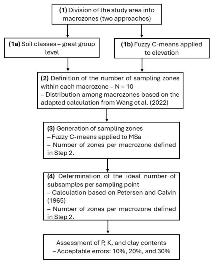
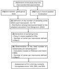
The research workflow can be described in four main steps. (1) First, the study area was divided into macro-zones through a spatial blocking scheme using two distinct approaches: (1a) delineation based on soil classes at the great group level; and (1b) application of the Fuzzy C-Means (FCM) algorithm to the Digital Elevation Model (DEM), supported by the Fuzzy Performance Index (FPI) and the Modified Partition Entropy (MPE), resulting in elevation-based macro-zones. (2) The number of sampling zones (predefined as N = 10 for the entire area) was proportionally distributed among the macro-zones according to an equation adapted from Wang et al. (2023), accounting for internal variability and macro-zone size. (3) Next, the Fuzzy C-Means algorithm was applied again—this time to the raster of soil apparent magnetic susceptibility (MSa) within each macro-zone—to define the sampling zones (micro-regions), meeting the previously stipulated number of zones. (4) Finally, the ideal minimum number of subsamples to compose a representative sample of phosphorus (P), potassium (K), and clay was determined using the equation proposed by Petersen & Calvin (1965), adopting three acceptable error thresholds: 10%, 20%, and 30%. A schematic representation of this sampling approach is presented in Figure 1.

Figure 1
Research workflow.

Study area

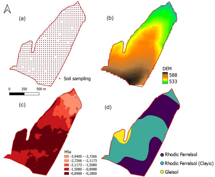
The study area covers 107 hectares and is located in the municipality of Cosmópolis, São Paulo State, Brazil, at 22°41′55.16″S, 47°10′34.15″W (Figure 2). The climate is classified as Cwa—humid subtropical with a hot summer—according to Köppen, with a mean annual precipitation of 1,400 mm and a

Figure 2
Study area showing: dense-grid sampling points (a), digital elevation model (b), soil apparent magnetic susceptibility (c), and soil classes (d).

mean annual temperature of 20–22°C. The relief is gently undulated and the soil is predominantly a Latossol (Oxisol), with surface (0–20 cm) texture classes ranging from clay to loam–clay–sand. Grain cropping predominates in the area, with soybean in the first season, alternating between oat and grain sorghum in the second season.

Soil sampling

Across the entire study area, dense soil sampling was conducted using a regular 40 × 40 m grid, corresponding to 6 sampling points per hectare (Figure 2a). Each sampling point represents a composite sample formed from six subsamples collected within a 5 m radius of the central point using an instrumented quad bike equipped with an automated auger. The sampling dataset is available in Melo & Amaral (2024). Samples were collected at a depth of 0–20 cm, as recommended for fertilizer prescription in grain-producing areas (Cantarella et al., 2022). This high sampling density enabled us to

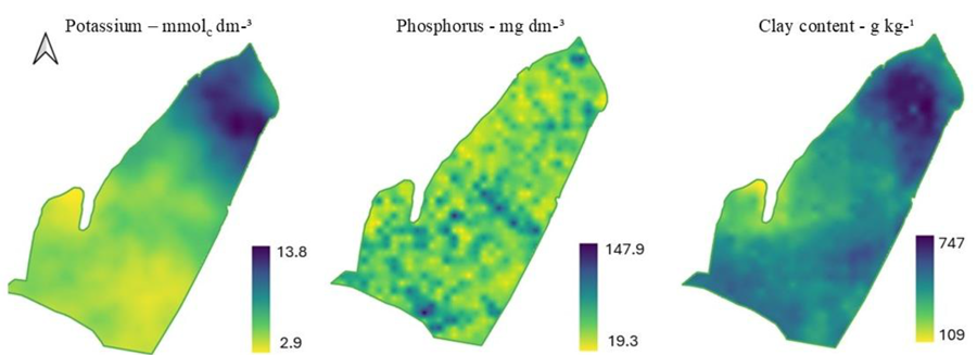
simulate several sampling configurations within the area. The composite samples were sent to a commercial soil testing laboratory for chemical and physical analyses. For this study, we selected three soil attributes: available phosphorus (P; mg dm⁻³), available potassium (K; mmolc dm⁻³), and soil texture represented by clay content (g kg⁻¹) (Figure 3). Descriptive statistics for these attributes are provided in Table 1. Phosphorus and potassium were chosen because they are the nutrients most frequently replenished by fertilization in agricultural areas, while clay was included due to its influence on soil fertility through its relation with cation exchange capacity (CEC) and water storage.

Figure 3
Spatial distribution maps for the study variables (available P and K, and clay content).

Table 1
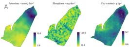
Descriptive statistics (n = 650) and degree of spatial clustering estimated by Moran’s I for available phosphorus (mg dm⁻3), potassium (mmolc dm⁻3), and clay content (g kg⁻1).

Soil property	Mean	Median	Std. Dev.	C. Var. (%)	Min	Max	Moran´s Index
Potassium, K	6.0	5.3	3.0	50.5	0.8	19.3	0.66
Phosphorus, P	50.5	45	23.5	46.5	13	164	0.2
Clay content	460.5	459	108.6	23.5	108	750	0.85

Environmental covariates

The proposed methodology aimed to infer variability in the study areas through soil macro- and micro-variability, a strategy used by Wang et al. (2023) and Melo et al. (2025). The purpose of dividing the area into macro-zones is to use a block-like scheme that enables the identification of homogeneous zones at a broader scale. This approach helps reduce part of the field variability and then allows these zones to be subdivided into micro-regions. These micro-regions are defined as the sampling zones, which serve as the fine-tuning step to reduce variability across the sampled area, enabling the collection of subsamples that faithfully represent the attributes of interest within each zone, thereby ensuring improved efficiency in variable-rate fertilizer application.

For this study, we tested two scenarios for delineating macro-zones: soil taxonomic classes (Figure 1d; EMBRAPA SOLOS, 2018), which provide fundamental information for grouping regions with similar soil characteristics; and elevation derived from the digital elevation model (DEM), following the original proposal of Wang et al. (2023). The DEM was obtained directly from the Google Earth Engine platform (Copernicus DEM), whose original imagery is available at 30 m spatial resolution and was subsequently resampled to 10 m using the bilinear method (Figure 1b). The suite of DEM-derived variables has been widely investigated for soil class mapping (Bazaglia Filho et al., 2013; Brungard et al., 2015; Ma et al., 2019) and for digital soil mapping (DSM) (Wang et al., 2023; An et al., 2018), which justifies its use in this project as an alternative to soil class maps, given that producers do not always have access to farm-scale soil class mapping.

The covariate used to delineate the micro-regions—corresponding to the sampling zones—was soil apparent magnetic susceptibility (MSa), an attribute that has proven effective for identifying site-specific management zones (Melo et al., 2025; Matos et al., 2023). In addition, MSa has been employed in soil studies for attribute prediction (Ramos et al., 2021), to support mapping (Pusch et al., 2023), and to refine the delineation of boundaries between different soil classes (Silva Junior et al., 2021). In seemingly homogeneous areas, MSa can reveal subtle variations due to its association with soil mineralogy, enabling separation into zones of interest that may exhibit different levels of soil fertility. MSa data were acquired for a depth of up to 37.5 cm using a real-time electromagnetic induction instrument (EM38-MK2, Geonics Ltd., Canada). The instrument was towed by a quad bike along passes spaced 30 m apart, resulting in a data-collection density of approximately 150 readings per hectare. A continuous raster was subsequently produced through ordinary kriging (Figure 1c).

Delineation of sampling zones

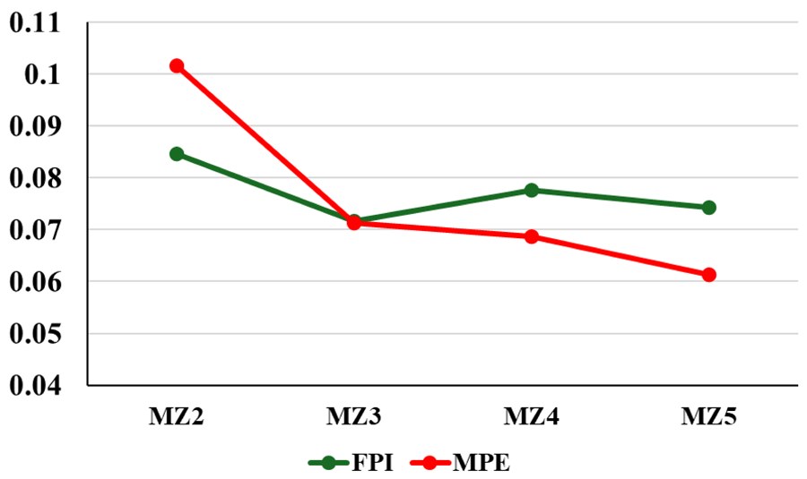
For the scenario using soil classification as the primary information to delineate macro-zones, the file was produced in vector format by a specialist pedologist, and the number of macro-zones corresponded to the number of soil classes defined down to the great group level, resulting in three macro-zones. In the case in which the DEM served as the primary information, because it is a raster without predefined classes, we classified it using fuzzy C-Means clustering (Córdoba et al., 2016; Oldoni et al., 2019). The selection of the optimal number of macro-zones was based on the joint analysis of the Fuzzy Performance Index - FPI (McBratney & Moore, 1985) and the Modified Partition Entropy - MPE (Boydell & McBratney, 2002), which have been used in studies for defining management zones (Melo et al., 2025; Oldoni et al., 2025; Oldoni et al., 2019). Three DEM clusters were identified as optimal, as this was the clustering level at which both indices were low, particularly the FPI (Figure 4), resulting in three macro-zones (Figure 5). Finally, we applied the majority (mode) filter in the Precision Zones plugin (11×11-pixel window) to reduce salt-and-pepper noise, removing small pixel clusters of one zone embedded within another and making the map more continuous and operational (Melo et al., 2025).

Figure 4
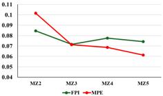
Fuzzy Performance Index (FPI) and Modified Partition Entropy (MPE) used to select the optimal number of macro-zones, showing results from two (MZ2) to five (MZ5) clusters.

Figure 5
Macro-zones created through DEM elevation using Fuzzy C-Means clustering.

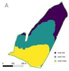
The optimal number of sampling zones within each macro-zone (soil class or elevation—DEM) was determined as a function of MSa variability and class area (Eq. 1). The basic premise is that greater variability in MSa likely reflects greater variability in soil attributes. The equation adapted from Wang et al. (2023), which determines the number of soil sampling zones within each macro-zone, starts from an arbitrarily defined number of samples—which commonly occurs in field practice, typically constrained by the available budget. In this study, we assumed the budget was limited to ten samples for the entire area, providing zones with an average area of ~10 ha, which falls within the range recommended for conventional soil sampling in agriculture (Cantarutti et al., 2007; van Raij, 2017). The sampling zones within each macro-zone were created using the fuzzy C-means clustering method, as in Melo et al. (2025). Noise filtering was performed as previously described for the macro-zone segmentation (Melo et al., 2025).

${\mathrm{SN}}_n=\mathrm{SN}\cdot A_n\cdot \mathrm{CVh}/\sum \mathrm{Ah}\cdot {\mathrm{CV}}_n$

Where:

SNh – Number of sampling zones in each macro-zone.

SN – Number of sampling points to be targeted across the entire area, arbitrarily defined (n = 10).

Ah – Area of each macro-zone under study (ha).

CVh – Coefficient of variation of apparent magnetic susceptibility (MSa) in each macro-zone.

Determination of the optimal number of subsamples

After delineating the sampling zones, we sought to infer the optimal number of soil subsamples needed to represent the mean values for clay, P, and K based on the reference-grid sampling points located within each zone. The optimal number of subsamples was determined using [eq. (2)], as proposed by Petersen & Calvin (1965). We adopted a 5% significance level, and the optimal number of subsamples for each sampling point was computed considering maximum allowable errors of 10%, 20%, and 30% relative to the mean, as in Pias et al. (2018).

$n=\left(\right(t\cdot S)/D{)}^2$

Where:

n = required number of subsamples

t = Student’s *t* distribution value for the significance level (α) and degrees of freedom (DF) in each sampling zone (DF = number of samples in the sampling zone − 1).

S = sample standard deviation of each attribute measured within each sampling zone.

D = mean of each attribute within the sampling zone divided by the allowable percentage variation around the mean (10%, 20%, and 30%).

Analysis of the results

The clustering of sampling points within each of the two sampling-zone configurations was assessed visually using boxplots and compared with the entire dataset for the full area, considered here as the conventional approach. Next, we calculated the optimal number of sampling points with the corresponding allowable sampling errors (10%, 20%, and 30%—Equation 2) for each sampling zone, enabling the determination of the ideal number of subsamples per zone. The two macro-zone configurations were then compared based on the mean optimal number of subsamples required in each sampling zone, in order to identify the one with better performance in terms of homogeneity and reduced ideal number of subsamples. To explore potential relations among the evaluated attributes, we computed Spearman’s correlation between MSa and the tested soil attributes to help explain possible discrepancies among results (Figure 8). Finally, we evaluated zone homogeneity considering the recommended optimal number of subsamples and compared these values with the mean of all sampling points within each zone, used as the reference.

Figure 8
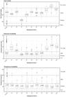
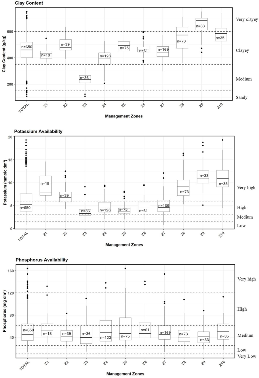
Distribution of subsample values for soil attributes in the ten zones defined based on soil classes (macro-zones) and apparent magnetic susceptibility (MSa—micro-zones), compared with the complete set of samples collected across the entire area (TOTAL). Dashed axes indicate nutrient availability classes and texture classes as a function of soil clay percentage (adapted from Cantarella et al., 2022).

Results and Discussion

Partitioning the agricultural field into macro-zones and subsequently into sampling zones enabled efficient mapping under both scenarios tested. In total, we obtained 10 sampling zones in each macro-zone delineation configuration (Figure 6). For the soil-class configuration, we obtained four zones in macro-zone 1, five in macro-zone 2, and one in macro-zone 3. For the configuration based on DEM elevation, clustering provided four sampling zones in zone 1, four in zone 2, and two in zone 3. Regarding the ideal minimum number of subsamples per zone, the results indicated that approximately 12 subsamples are needed to characterize the tested attributes in each zone, regardless of MZ size. Another important point is that using the DEM to subdivide the area into macro-zones can be a practical alternative, since several producers lack detailed pedological mapping available, which could otherwise limit adoption of the technique. These findings underscore the need to tailor sampling strategies to maximize mapping accuracy and optimize available resources for efficient management.

Figure 6
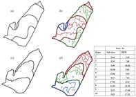
Soil sampling zones (b & d) with their respective areas indicated in the adjacent table: macro-zones generated from the three soil classes (a) and their respective sampling zones derived from soil apparent magnetic susceptibility (MSa) (b); three macro-zones generated from DEM elevation (c) and their respective sampling zones derived from soil apparent magnetic susceptibility (MSa) (d).

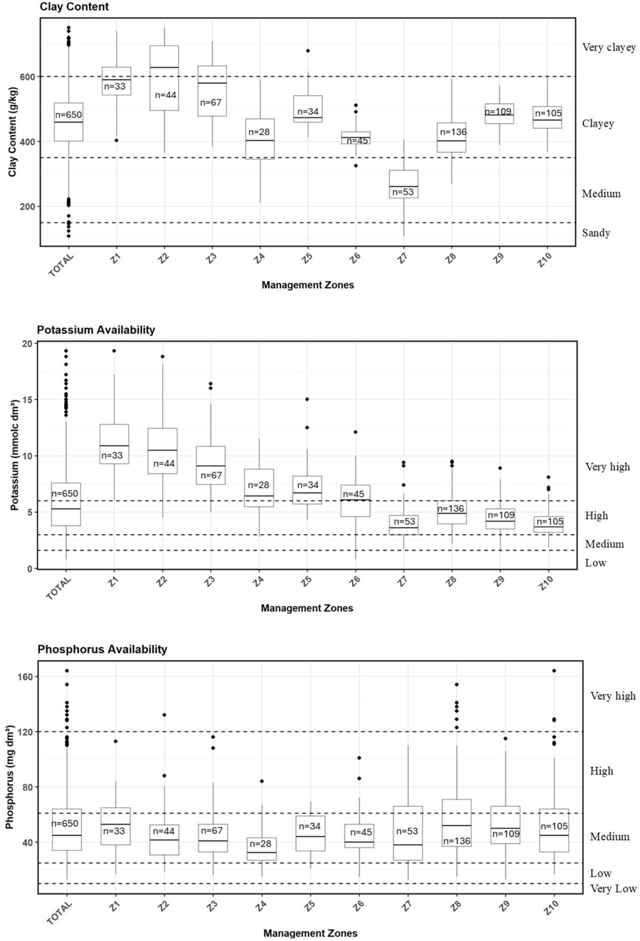
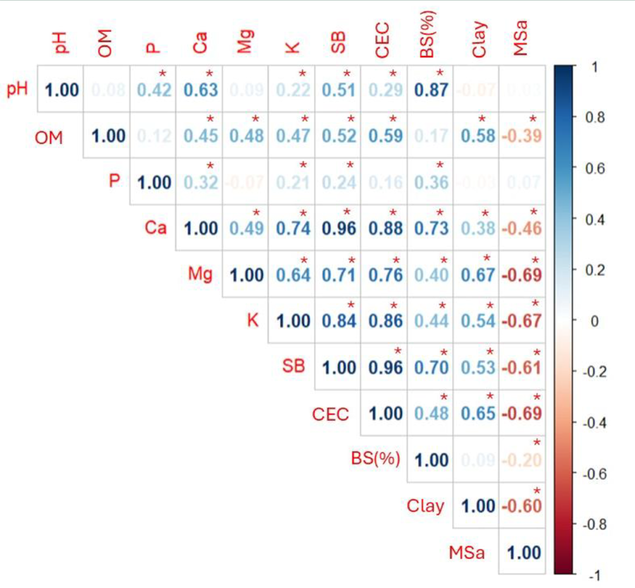
Dividing the area into ten sampling zones reduced the variability of clay and potassium data across all zones when compared with the full dataset that would represent conventional sampling, regardless of the variable used to delineate the macro-zones of homogeneity. This can be observed in the boxplots of Figures 7 and 8: for the complete set of soil samples (n = 650), once the area was partitioned into ten zones, the boxplots became less dispersed, indicating greater within-zone homogeneity for both attributes. For clay, both methods for creating macro-zones (soil classes and DEM elevation) provided four out of ten zones with 100% of points falling within the same textural class, while six zones had at least 75% of points in the same class (Figures 7 and 8). For potassium, delineating macro-zones based on soil classes produced two zones with 100% of points within the same level, five zones with 75% of points at the same level, and all zones with at least 50% of points at the same level (Figure 8). In contrast, zones generated from the DEM resulted in one zone with 100% of points at the same level, four zones with 75%, and the remaining five zones with 50% (Figure 7). Because the MZ strategies effectively reduced dispersion for clay and K, variables that exhibited spatial clustering (Table 1) and correlated with nearly all analyzed attributes (organic matter = OM, base saturation = SB(%), cation exchange capacity = CEC, calcium = Ca, and magnesium = Mg), except P and pH (Figure 9), we consider this subdivision approach suitable for characterizing soil chemical fertility in the study area.

Figure 7
Distribution of subsample values for soil attributes in the ten zones defined based on elevation (DEM—macro-zones) and apparent magnetic susceptibility (MSa—micro-zones), compared with the complete set of samples collected across the entire area (TOTAL). Dashed axes indicate nutrient availability classes and texture classes as a function of soil clay percentage (adapted from Cantarella et al., 2022).

Figure 9
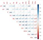
Spearman’s correlation among soil attributes (K = available potassium, P = available phosphorus, Ca = exchangeable calcium, Mg = exchangeable magnesium, Clay = clay content, SB(%) = base saturation, CEC = cation exchange capacity, SB = sum of bases, OM = organic matter, pH = hydrogen potential, MSa = apparent magnetic susceptibility). \* = Significant at the 5% level (n = 650).

Regarding available soil phosphorus, the zoning approaches were not effective at reducing within-zone variability, with boxplots exhibiting distributions similar to those of the full dataset and across zones (Figures 7 and 8). As shown in Figures 7 and Figure 8, seven of the zones contained only 50% of the data within the same availability level, regardless of the method used. This behavior can be attributed to the low mobility of phosphorus in the soil profile and the high fertilization demand for this nutrient (Cantarella et al., 2022), factors that contribute to its high randomness and variability—corroborated by a non-significant Moran’s I for P (Table 1). This indicates that, in this study area, delineating sampling zones did not assist in mapping available P. However, mapping attributes with weak spatial dependence is particularly challenging even under grid sampling, which hampers variogram estimation (Melo et al., 2025; Amaral & Justina, 2019) and negatively affects interpolation for map creation. Given this limitation, a conventional sampling strategy representing the entire area could be used here. Nevertheless, although zoning did not aid P mapping in this field, it did not impair it either, and it remains a safe approach that may deliver results in other areas and has demonstrably helped with other attributes such as K and clay noted above.

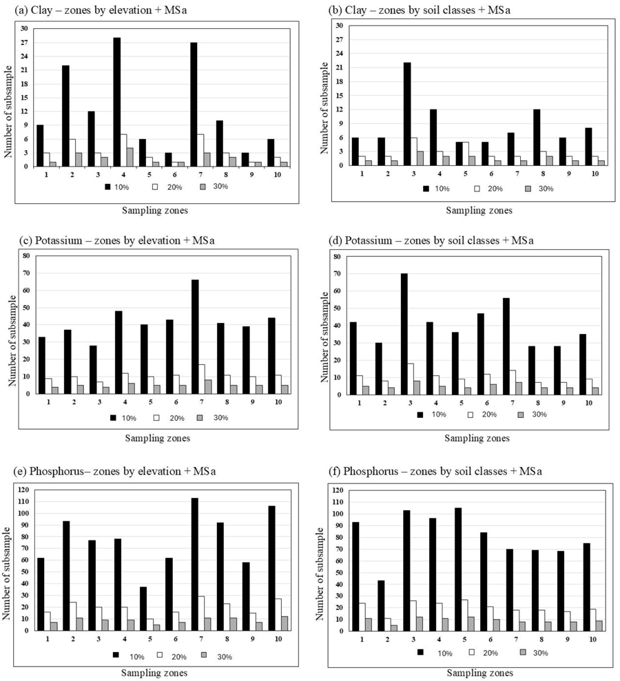
The size of the sampling zones obtained by the different methods had no influence on the number of soil subsamples required to represent each zone. For the zones generated based on soil classes, four were larger than 10 hectares, while six were smaller. In contrast, the distribution was reversed for zones delineated by elevation, with six zones smaller than 10 hectares and four larger (Figure 6). For example, zone 3—defined from soil classes—has approximately 5 hectares and required the highest number of subsamples for clay and K (22 and 70, respectively) for an allowable error of 10% (Figures 10b and 10d). Conversely, zone 7—also delineated by soil classes—with about 27 hectares, demanded only one-third of that number to characterize clay at the same allowable error (Figure 10b). Zone 3 (Figure 6b) was delineated by soil classes and, due to its small size and the variability of MSa, it received only one sampling zone within its class (Entisols) according to the calculation of Wang et al. (2023). This zone (3) showed highly discrepant subsample requirements relative to the others (Figures 10b and 10d) because it encompassed the Entisols (Figure 2d), which naturally exhibits high variability due to fluctuations in the water table. This phenomenon affects redox processes, altering nutrient availability (Guimarães et al., 2013) and requiring a greater number of subsamples for representative sampling. This same pattern—namely, no relation between zone size and subsample needs, to greater or lesser degrees—can be extended to all zones under both delineation methods. Thus, working with a fixed number of subsamples per sampling zone appears appropriate, especially since within-macro-zone variability was reduced by grouping micro-zones based on soil apparent magnetic susceptibility (MSa).

Figure 10
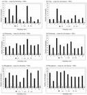
Number of subsamples per sampling zone required to estimate soil clay, potassium, and available phosphorus with maximum errors of 10%, 20%, and 30% relative to the mean, considering different zoning criteria: (a, b) clay in zones delineated by elevation + MSa and by soil classes + MSa, respectively; (c, d) potassium in zones delineated by elevation + MSa and by soil classes + MSa; (e, f) phosphorus in zones delineated by elevation + MSa and by soil classes + MSa.

Although both delineation approaches reduced data variability (Figures 7 and 8), they led to different numbers of subsamples needed to efficiently represent the attributes within zones (Figure 10), and these differences were unrelated to either zone area or MSa variability. Because the two zoning methods produced distinct zone areas and boundaries, examining the subsample counts for each zone individually precludes inferring a single per-zone sample size or determining which delineation provided better clustering of data. Thus, a sound strategy is to adopt an average number of subsamples across zones within each sampling configuration—one that is feasible to collect in the field and adequately represents most attributes of interest. As discussed above, the spatial pattern of phosphorus was not adequately captured by the sampling zones and was therefore removed from the analysis. Using soil classes to delineate macro-zones produced sampling zones that were more homogeneous in terms of K and clay contents, as evidenced by the lower mean subsample requirement (Figure 11) relative to elevation-based zones. This greater efficiency of soil-class-based macro-zones may be associated to expert-driven delineation, which, despite its subjectivity (Bazaglia Filho et al., 2013), involves field investigation and renders zones more representative. Moreover, terrain attributes are not always ideal for inferring surface soil properties (Nalin et al., 2023). Hence, using soil classes proved a more effective approach for grouping sampling zones and provides an additional application for detailed pedological surveys in agricultural areas.

Figure 11
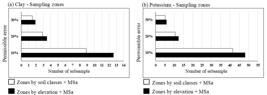
Average number of subsamples required to represent soil attributes as a function of error thresholds (10%, 20%, and 30%) according to the sampling-zone delineation methods: elevation plus apparent magnetic susceptibility (MSa) shown in white, and soil-class-based zones plus apparent magnetic susceptibility (MSa) shown in black.

Because clay content in the area exhibits stronger spatial clustering than available K (higher Moran’s I—Table 1), its subsample demand was lower: 9, 3, and 2 subsamples in the zones delineated by soil classes, while potassium required 41, 11, and 5 subsamples, corresponding to allowable errors of 10%, 20%, and 30% of the mean, respectively. The interpolated maps (Figure 3) highlight the spatial variability of the two evaluated attributes. Clay shows a more continuous pattern, indicating greater homogeneity, whereas potassium (K) shows greater spatial discontinuity, possibly associated with anthropogenic management and the intrinsic variability of chemical attributes at smaller scales—thereby corroborating the differing subsample requirements within zones for the two attributes. Since it is common to perform a single sampling to analyze a suite of attributes (i.e., P, K, pH, texture, Ca, Mg, etc.), to ensure reliable representation of all of them, the minimum number of subsamples can be set based on the attribute that required the highest quantity. Assuming an acceptable error of 10%, the subsample demand would be very high—namely, at least 41 subsamples for accurate determination of soil K (Figure 11). Such number would render sampling excessively expensive due to the operational costs of soil collection. Thus, even though it could provide good results, such sampling density becomes operationally unfeasible.

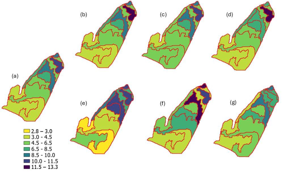
Adopting allowable errors of 20% and 30% substantially reduced the number of subsamples needed to stabilize the mean K value—from 12 and 4 subsamples in the elevation-derived zones to 11 and 3 in the soil-class-based zones, respectively (Figure 11b)—, which is close to guidance for subsampling homogeneous fields under the traditional “mean-based” approach (Cantarutti et al., 2007; van Raij, 2017). Thus, assuming a 20% acceptable error provides practical results: for example, if the mean K in a zone is 4.9 mmolc dm⁻³, then with a 20% error the values range from 3.92 to 5.88 mmolc dm⁻³, maintaining the same nutrient-availability class (High = 3.1–6.0 mmolc dm⁻³). By contrast, with a 30% error, this same example would range from 3.43 to 6.37 mmolc dm⁻³, which would already fall outside the same availability class (Very high > 6.0 mmolc dm⁻³), compromising decision-making (Cantarella et al., 2022). To assess the stability of zone mean representation, we simulated three subsampling scenarios, randomly selecting 12 samples from each zone to compare the resulting K maps—i.e., assuming a maximum error of 20%. When examining the available-potassium maps, there was virtually no difference among the simulations, nor any relevant difference compared with the map generated from all subsamples (reference grid, n = 650) (Figure 12). In contrast, when we ran the same simulations using only 4 subsamples—the number that would be ideal for the attribute with lower variation (clay), also at a 20% error—the resulting maps showed markedly different K values for the same zones (Figure 12). This reinforces that, in the case of a single sampling to represent multiple attributes, the number of subsamples should follow the requirement of the attributes with the greatest variability. For illustration, zone 5 (generated from elevation + MSa) has a reference mean K of 7.2 mmolc dm⁻³; however, with a reduced number of subsamples (n = 4), the means ranged from 5.45 to 10.17 mmolc dm⁻³ (data not shown). In this situation, values varied by approximately +41.25% and −24.31% relative to the mean of all samples within the zone, which would alter the nutrient-availability class when compared with technical bulletins and fertilization manuals, leading to erroneous fertilizer recommendations. Therefore, to achieve efficient mapping results, it is necessary to follow the recommendation of a minimum of 12 subsamples, thereby avoiding potential overestimation or underestimation of values within the sampling zones.

Figure 12
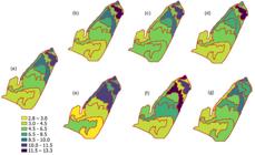
Sampling zones generated from elevation (DEM) and apparent magnetic susceptibility (MSa) showing mean values of available potassium in the soil (mmolc dm⁻3): (a) mean of all sampling points (reference); (b, c, d) mean K from simulations of distinct walking paths with 12 subsamples (recommended) per zone; (e, f, g) mean K from simulations with only 4 subsamples for comparison.

Conclusions

Soil classes are slightly more effective than elevation for delineating macro-zones within the experimental area. However, detailed pedological classification is still uncommon on farms because it requires an expert with tacit knowledge and field visits. Alternatively, using more readily available data, such as elevation, emerges as a viable option for generating sampling zones.

Management zone-based sampling using apparent magnetic susceptibility to define micro-zones and consequently characterize multiple soil attributes enables grouping areas with similar characteristics for attributes that exhibit spatial clustering. However, the proposed methodology becomes inefficient for mapping attributes that lack spatial clustering (as with phosphorus in this study), though it does not preclude or undermine its use.

Although soil attributes tend to exhibit some degree of interrelation, each shows a minimally distinct spatial behavior, meaning there is no single number of subsamples that is suitable for all; it varies according to spatial clustering and the magnitude of variation. Because soil sampling usually targets a suite of attributes rather than a single one, the minimum number of subsamples for a composite sample should be determined based on the attribute that requires the largest sample size to represent the mean within the zone. In this experiment, we tested three error levels (10%, 20%, and 30%) relative to the mean of all points. Since fertilizer prescriptions follow technical bulletins that classify nutrient availability into a few ranges, small deviations in the estimated zone mean would not change the final recommendation. However, variations up to 10% may represent an overly fine adjustment that would greatly increase sampling costs (n > 41). Therefore, balancing survey quality and operational complexity, a 20% error threshold appears more appropriate, providing a feasible number of subsamples, close to what is traditionally used (between 10 and 20). Using 30% may cause coarser shifts among nutrient-availability levels, potentially affecting soil fertility diagnosis and fertilizer recommendations. Accordingly, a subsample count close to 12 seems adequate for accurately representing the mean value of each zone, regardless of its size. However, this may vary depending on the variability levels of the measured attributes, thus justifying studies under diverse conditions.

Acknowledgments

We gratefully acknowledge the São Paulo Research Foundation (FAPESP) for the first author’s scholarship (grant no. 2024/14044-4) and the Brazilian Federal Agency for Support and Evaluation of Graduate Education (CAPES) — Finance Code 001 — for the second author’s scholarship. This research was supported by FAPESP (grant no. 2022/03160-8). We also thank Fazenda São José for providing the study area, without which this research would not have been possible.

REFERENCES

• Amaral, L. R. D., & Justina, D. D. D. (2019). Spatial dependence degree and sampling neighborhood influence on interpolation process for fertilizer prescription maps. Engenharia Agrícola, 39, 85-95.
• Ameer, S., Cheema, M. J. M., Khan, M. A., Amjad, M., Noor, M., & Wei, L. (2022). Delineation of nutrient management zones for precise fertilizer management in wheat crop using geo-statistical techniques. Soil use and Management, 38 (3), 1430-1445.
• An, Y., Yang, L., Zhu, A. X., Qin, C., & Shi, J. (2018). Identification of representative samples from existing samples for digital soil mapping. Geoderma, 311, 109-119.
• Bazaglia Filho, O., Rizzo, R., Lepsch, I. F., Prado, H. D., Gomes, F. H., Mazza, J. A., & Demattê, J. A. M. (2013). Comparison between detailed digital and conventional soil maps of an area with complex geology. Revista Brasileira de ciência do solo, 37, 1136-1148.
• Brungard, C. W., Boettinger, J. L., Duniway, M. C., Wills, S. A., & Edwards Jr, T. C. (2015). Machine learning for predicting soil classes in three semi-arid landscapes. Geoderma, 239, 68-83.
• Brus, D. J. (2019). Sampling for digital soil mapping: A tutorial supported by R scripts. Geoderma, 338, 464-480.
• Boydell, B., & McBratney, A. B. (2002). Identifying potential within-field management zones from cotton-yield estimates. Precision agriculture, 3, 9-23.
• Cantarella, H., Raij, B. Van, Quaggio, J. A., Boaretto, R. M., & Mattos, D. (2022). Recomendação de adubação e calagem para o Estado de São Paulo. Instituto Agrônomico de Campinas.
• Cantarutti, R. B., Barros, N. F. de, Prieto, H. E., & Novais, R. F. (2007). Avaliação da fertilidade do solo e recomendação de fertilizantes. In R. F. Novais et al. (Orgs.), Fertilidade do solo (pp. 769-850). Sociedade Brasileira de Ciência do Solo.
• Cherubin, M. R., Damian, J. M., Tavares, T. R., Trevisan, R. G., Colaço, A. F., Eitelwein, M. T., Martello, M., Inamasu, R. Y., Pias, O. H. d. C., & Molin, J. P. (2022). Precision agriculture in Brazil: the trajectory of 25 years of scientific research. Agriculture, 12(11), 1882.
• Cherubin, M. R., Santi, A. L., Eitelwein, M. T., Amado, T. J. C., Simon, D. H., & Damian, J. M. (2015). Dimensão da malha amostral para caracterização da variabilidade espacial de fósforo e potássio em Latossolo Vermelho. Pesquisa Agropecuária Brasileira, 50, 168-177.
• Córdoba, M. A., Bruno, C. I., Costa, J. L., Peralta, N. R., & Balzarini, M. G. (2016). Protocol for multivariate homogeneous zone delineation in precision agriculture. Biosystems engineering, 143, 95-107.
• Doerge, T. A. (1999). Management zone concepts (SSMG-2). Potash & Phosphate Institute.
• EMBRAPA. (2018). Sistema brasileiro de classificação de solos. Empresa Brasileira de Pesquisa Agropecuária.
• Gebbers, R., & Adamchuk, V. I. (2010). Precision agriculture and food security. Science, 327 (5967), 828-831.
• Ghotbi, A. R., & Taciroglu, E. (2021). Structural seismic damage and loss assessments using a multi-conditioning ground motion selection approach based on an efficient sampling technique. Bulletin of Earthquake Engineering, 19, 1271-1287.
• Guimarães, S. T., Lima, H. N., Teixeira, W. G., Neves Junior, A. F., Silva, F. W. R., Macedo, R. S., & Souza, K. W. D. (2013). Caracterização e classificação de gleissolos da várzea do rio Solimões (Manacapuru e Iranduba), Amazonas, Brasil. Revista Brasileira de Ciência do Solo, 37, 317-326.
• Kerry, R., Ingram, B., Oliver, M., & Frogbrook, Z. (2024). Soil sampling and sensed ancillary data requirements for soil mapping in precision agriculture I. delineation of management zones to determine zone averages of soil properties. Precision Agriculture, 25 (3), 1181-1211.
• Kountios, G., Ragkos, A., Bournaris, T., Papadavid, G., & Michailidis, A. (2018). Educational needs and perceptions of the sustainability of precision agriculture: Survey evidence from Greece. Precision Agriculture, 19, 537-554.
• Ma, Y., Minasny, B., Malone, B. P., & Mcbratney, A. B. (2019). Pedology and digital soil mapping (DSM). European Journal of Soil Science, 70 (2), 216-235.
• Matos, A. P. D., Matias, S. S. R., Nunes, R. K. L., Morais, E. M., & Tavares Filho, G. S. (2023). Soil management of limed areas cultivated with banana identified by magnetic susceptibility. Revista Ceres, 70, 17-24.
• Mazur, P., Gozdowski, D., & Wójcik-Gront, E. (2022). Soil electrical conductivity and satellite-derived vegetation indices for evaluation of phosphorus, potassium and magnesium content, pH, and delineation of within-field management zones. Agriculture, 12 (6), 883.
• McBratney, A. B., & Moore, A. W. (1985). Application of fuzzy sets to climatic classification. Agricultural and forest meteorology, 35 (1-4), 165-185.
• Melo, D. D., Cunha, I. A., & Amaral, L. R. (2025). Hierarchical Stratification for Spatial Sampling and Digital Mapping of Soil Attributes. AgriEngineering, 7 (1).
• Melo, D. D., & Amaral, L. R. do. (2024). Replication data for: Hierarchical stratification for spatial sampling and digital mapping of soil atributes. https://doi.org/10.25824/redu/8QITE4
  » https://doi.org/10.25824/redu/8QITE4
• Nalin, RS, Dalmolin, RSD, de Araújo Pedron, F., Moura-Bueno, JM, Horst, TZ, Schenato, RB, & Soligo, MF (2023). Contabilização da variação espacial do fósforo disponível explicada por covariáveis ??ambientais. Geoderma Regional, 32, e00594.
• Oldoni, H., Magalhães, P. S., Oliveira, A. L., Lima, J. P., Figueiredo, G. K., Moro, E., & Amaral, L. R. (2025). Management zones delineation: a proposal to overcome the crop-pasture rotation challenge. Precision Agriculture, 26 (1), 21.
• Oldoni, H., Terra, V. S. S., Timm, L. C., Júnior, C. R., & Monteiro, A. B. (2019). Delineation of management zones in a peach orchard using multivariate and geostatistical analyses. Soil and Tillage Research, 191, 1-10.
• Petersen, R. G., & Calvin, L. D. (1965). Sampling. In C. A. Black (Ed.), Methods of soil analysis: Physical and mineralogical properties, including statistics of measurement and sampling (pp. 54-71). American Society of Agronomy.
• Pias, O. H. D. C., Cherubin, M. R., Basso, C. J., Santi, A. L., Molin, J. P., & Bayer, C. (2018). Soil penetration resistance mapping quality: effect of the number of subsamples. Acta Scientiarum. Agronomy, 40, e34989.
• Pusch, M., Samuel-Rosa, A., Magalhães, P. S. G., & do Amaral, L. R. (2023). Covariates in sample planning optimization for digital soil fertility mapping in agricultural areas. Geoderma, 429, 116252.
• Ramos, P. V., Inda, A. V., Barrón, V., Teixeira, D. D. B., & Marques Jr, J. (2021). Magnetic susceptibility in the prediction of soil attributes in southern Brazil. Soil Science Society of America Journal, 85 (1), 102-116.
• Silva Junior, J. F., Siqueira, D. S., Teixeira, D. D. B., Panosso, A. R., Júnior, J. M., & Pereira, G. T. (2021). Multivariate split moving windows and magnetic susceptibility for locating soil boundaries of São Paulo, Brazil. Geoderma Regional, 26, e00418.
• Tripathi, R., Tripathy, B. R., Gouda, A. K., Swain, C. K., Mohanty, S., & Nayak, A. K. (2024). Delineating Homogeneous Management Zones for Nutrient Management in Rice Cultivated Area of Eastern India. Journal of Soil Science and Plant Nutrition, 24 (4), 8331-8342.
• Trivedi, M. B., Bates, T. R., Meyers, J. M., Shcherbatyuk, N., Davadant, P., Chancia, R., ... & Heuvel, J. V. (2025). Box sampling: a new spatial sampling method for grapevine macronutrients using Sentinel-1 and Sentinel-2 satellite images. Precision Agriculture, 26 (2), 35.
• Valente, D. S. M., Pereira, G. W., de Queiroz, D. M., Zandonadi, R. S., Amaral, L. R. d., Bottega, E. L., Costa, M. M., de Freitas Coelho, A. L., & Grift, T. (2024). Accuracy of Various Sampling Techniques for Precision Agriculture: A Case Study in Brazil. Agriculture, 14 (12), 2198.
• van Raij, B. (2017). Fertilidade do solo e manejo de nutrientes. IPNI.
• Wang, Y., Qi, Q., Bao, Z., Wu, L., Geng, Q., & Wang, J. (2023). A novel sampling design considering the local heterogeneity of soil for farm field-level mapping with multiple soil properties. Precision Agriculture, 24 (1), 1-22.

• Data Availability Statement:
  The datasets generated during and/or analyzed during the current study are available in the Research Data Repository of the University of Campinas (REDU/UNICAMP) repository, https://doi.org/10.25824/redu/8QITE4

Edited by

• Area Editor:
  Teresa Cristina Tarlé Pissarra

Data availability

The datasets generated during and/or analyzed during the current study are available in the Research Data Repository of the University of Campinas (REDU/UNICAMP) repository, https://doi.org/10.25824/redu/8QITE4

Publication Dates

• Publication in this collection
  02 Feb 2026
• Date of issue
  2026

History

• Received
  13 Apr 2025
• Accepted
  16 Sept 2025