Gauss-Newton Method Applied to Impedance Estimation in Grid-Connected Inverters

ABSTRACT

This work presents a methodology that employs the Gauss–Newton algorithm to perform online impedance estimation for grid-connected inverters. Conventional formulations for this class of problem typically lead to high-order nonlinear systems of equations, often of dimension 8×8. In contrast, the formulation proposed herein recasts the estimation task as a 3×3 least-squares problem, which is then solved via the Gauss–Newton method. To validate the proposed approach, a three-phase grid-connected inverter was adopted as the case study. The control system enforces three distinct active power injection levels into the grid, and the voltage, current, and phase-angle magnitudes at the point of common coupling are measured and used as inputs to the impedance estimation algorithm. Real-time validation was carried out to assess the performance of the method. The results confirm the feasibility of the proposed formulation and indicate that the approach substantially reduces the computational burden of embedded DSP-based algorithms for online grid impedance estimation.

KEYWORDS
Gauss-Newton method; grid impedance estimation; nonlinear least squares

I. INTRODUCTION

The massive integration of renewable energy sources, driven by global decarbonization targets by 2050, has transformed the profile of modern distribution grids [¹], [²]. This scenario has increased the density of grid-connected power electronic converters, making the investigation of interactions between the converter and grid impedance a critical factor for system stability. As discussed in [³], connecting distributed generation systems (DGS) to high-impedance grids can trigger dynamic instabilities and compromise power quality if control parameters are not properly adjusted.

Although power electronic converters typically operate reliably when connected to strong grids, the growing penetration of renewable energy sources is causing power systems to exhibit regions characterized by weak grid conditions (i.e., high grid impedance). Under these circumstances, the elevated grid impedance can interact with the inverter control system and the converter output impedance, potentially resulting in dynamic instabilities and degradation of power quality [⁴]. In this context, diagnostic tools are crucial for the real-time identification and characterization of such phenomena.

The grid impedance is not a static parameter; rather, it exhibits substantial temporal variability driven by load variations, the switching of capacitor banks employed for power factor correction, and grid reconfigurations [⁵]. Although impedance monitoring has traditionally been considered essential for high-power units (in the megawatt range) to guarantee global stability [⁶], it is becoming increasingly important for domestic-scale, low-power (some kilowatts) converters. In such distributed settings, the high density of power electronic converters can excite local harmonic resonances and cause failures in protection schemes if the control loops are not adaptively tuned to the time-varying grid impedance [⁷].

Grid impedance estimation techniques can be broadly classified into two principal categories [⁸]. The first category comprises non-invasive methods, which rely exclusively on measurements of voltages and currents to accomplish the estimation task. It should be emphasized, however, that the measured voltages and currents are inherently affected by any variations in the grid operating conditions, such as changes in load. Such variations must not occur within the time window and repetition rate required for accurate grid impedance estimation [⁹].

The second major category consists of the so-called invasive techniques, which rely on the deliberate application of controlled perturbations to the grid or to the control system [¹⁰]. These methodologies are particularly prevalent in the context of distributed generation systems, as the inverter itself can be used as a means of injecting such disturbances. Moreover, these approaches generally provide higher accuracy in the estimation of grid impedance [⁹], [¹¹].

Real-time grid impedance estimation has become an essential tool for adaptive control strategies, islanding detection, and filter resonance prevention [⁵]. Several methodologies have been explored in the literature, ranging from non-invasive techniques based on natural load variations to invasive methods that inject controlled disturbances to obtain more precise dynamic responses. Among the recent approaches, pseudo-random binary sequence (PRBS) injection [¹²], zero-sequence voltage injection [¹³], and the use of interpolated Fourier transforms [¹⁴] for phase extraction stand out.

One of the predominant origins of instability and power quality degradation in modern power systems is the dynamic interaction between the grid impedance and the inverter output impedance [⁴]. Contemporary power electronic converters continue to lack sufficiently advanced diagnostic methodologies for reliably identifying instability phenomena induced by variations in grid impedance. In this way, continuous monitoring and logging of the output voltages and currents at the point of common coupling (PCC) constitute a viable approach to facilitate accurate detection and analysis of such instability mechanisms [¹⁵].

Traditionally, the mathematical formulation for estimating grid RL parameters across multiple power levels yields high-order nonlinear systems, typically 8 × 8 [¹⁶], [¹⁷]. Although iterative methods such as Newton-Raphson, Potra-Pták, and Chun have proven effective in solving these systems, the computational cost associated with the recurrent calculation of large Jacobian matrices poses challenges for implementation in low-cost digital signal processors (DSPs) [¹⁸].

In this context, the objective of the present study is to formulate the problem as a 3 × 3 nonlinear least-squares adjustment. This reduction in the dimensionality of the problem substantially enhances the computational efficiency of digital signal processor DSP-embedded algorithms devoted to the real-time estimation of grid impedance.

To accomplish the stated objective, the developed formulation was integrated into the control architecture of a grid-connected three-phase inverter. The effectiveness of the proposed formulation was assessed by means of real-time simulations, in which performance indicators such as the percentage error of the estimated variables and the computational execution time were systematically analyzed.

The adoption of the proposed strategy is substantiated by the requirement for adaptive control schemes that operate with low latency, defined as the minimal delay between a control action and the corresponding system response. The reduction in the computational complexity of the impedance estimation algorithm developed in this study enhances the feasibility and efficiency of implementing these protection mechanisms in DSPs, thereby contributing to the preservation of system stability under variations in grid parameters. In addition, the reduced computational burden releases processing resources that can be allocated to other concurrent tasks.

The results demonstrate that the proposed formulation is effective, exhibiting reduced computational time and high estimation accuracy. Moreover, the reduced order of the formulation constitutes a significant contribution to the computational efficiency of algorithms designed for impedance estimation in grid-connected inverters.

II. TRADITIONAL FORMULATION

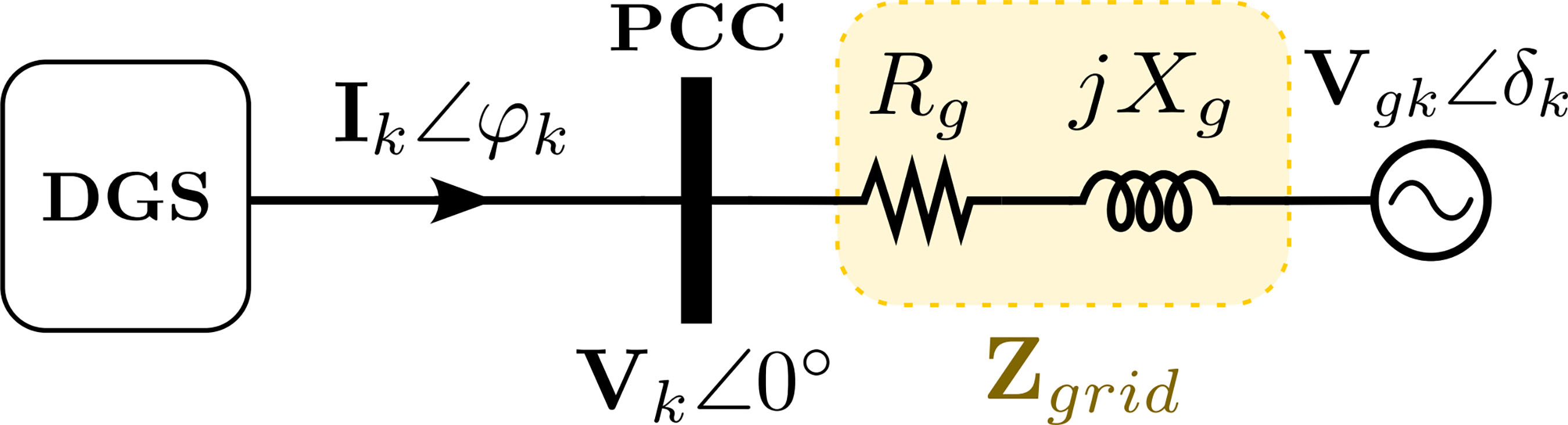
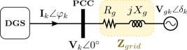
Fig. 1 depicts a generic grid-connected distributed generation system. In this configuration, the DGS injects a current phasor I_k∠φ_k into an electrical grid modeled as a Thevenin-equivalent voltage source V_gk∠δ_k in series with an impedance Z_grid = R_g + jX_g, where R_g and X_g denote, respectively, the resistance and the inductive reactance. The voltage at the PCC is represented by the phasor V_k∠0^◦. The subscript k is used to distinguish the different power levels that the DGS can inject into the grid.

By examining the variables depicted in Fig. 1, one can formulate:

FIGURE 1
Generic grid-connected distributed generation system.

(1) $V_{gk}\mathrm{\angle }{\delta }_k=V_k-(R_g+j{X}_g)I_k\mathrm{\angle }{\phi }_k$

Writing V_gk∠δ_k and I_k∠φ_k in rectangular form:

(2) $V_{gk}\mathrm{\angle }{\delta }_k=V_{gk}\cos {\delta }_k+j{V}_{gk}\sin {\delta }_k=V_{gkx}+j{V}_{gky}$

(3) $I_k\mathrm{\angle }{\phi }_k=I_k\cos {\phi }_k+j{I}_k\sin {\phi }_k=I_{kx}+j{I}_{ky}$

The subscripts x and y denote the real and imaginary components, respectively. By comparing (1) with (2) and substituting (3) into (1), we obtain the following expression:

(4) $\begin{array}{l}{V}_{gkx}+j{V}_{gky}=V_k-(R_g+j{X}_g)(I_{kx}+j{I}_{ky})\\ =V_k-R_g{I}_{kx}-j{R}_g{I}_{ky}-j{X}_g{I}_{kx}+X_g{I}_{ky}\\ =\underset{Real}{\underbrace{V_k-R_g{I}_{kx}+X_g{I}_{ky}}}-j\left(\underset{Imaginary}{\underbrace{R_g{I}_{ky}+X_g{I}_{kx}}}\right).\end{array}$

Upon comparing the respective sides of (4), we observe that:

(5) $\{\begin{array}{l}{V}_{gkx}=V_k-R_g{I}_{kx}+X_g{I}_{ky}\\ V_{gky}=-R_g{I}_{ky}-X_g{I}_{kx}\end{array}$

Considering three distinct levels of power injected into the grid by the DGS, system (5) can be reformulated as follows:

(6) $\{\begin{array}{l}{V}_{g1x}=V_1-R_g{I}_{1x}+X_g{I}_{1y}\\ V_{g1y}=-R_g{I}_{1y}-X_g{I}_{1x}\\ V_{g2x}=V_2-R_g{I}_{2x}+X_g{I}_{2y}\\ V_{g2y}=-R_g{I}_{2y}-X_g{I}_{2x}\\ V_{g3x}=V_3-R_g{I}_{3x}+X_g{I}_{3y}\\ V_{g3y}=-R_g{I}_{3y}-X_g{I}_{3x}\end{array}$

The instantaneous decomposition technique into sequence components (IDSC) presented in [¹⁹] uses as input the measurements of the voltage at the PCC and the current injected into the grid by the DGS. Application of this algorithm yields estimates of the PCC voltage amplitude (V_k) and of the amplitude (I_k) and phase angle (φ_k) of the current injected into the grid. Consequently, for each of the three distinct power injection levels, the quantities V₁, V₂, V₃, I_1x, I_1y, I_2x, I_2y, I_3x, and I_3y are known. Therefore, the system (6) consists of six equations with eight unknowns: V_g1x, V_g1y, V_g2x, V_g2y, V_g3x, V_g3y, R_g, and X_g.

It is reasonable to assume that the grid voltage amplitude (V_gk) does not undergo significant variations across the three distinct power injection levels provided by the DGS, i.e., V_g1 = V_g2 = V_g3. In other words, the magnitude of the phasor V_gk∠δ_k may be considered invariant during the application of the grid impedance estimation procedure. Considering that the magnitude of V_gk∠δ_k is

(7) $\left|V_{gk}\mathrm{\angle }{\delta }_k\right|=V_{gk}=\sqrt{V_{gkx}^2+V_{gky}^2},$

it can be expressed as:

(8) $V_{g1x}^2+V_{g1y}^2=V_{g2x}^2+V_{g2y}^2$

(9) $V_{g2x}^2+V_{g2y}^2=V_{g3x}^2+V_{g3y}^2$

The system (6) combined with (8) and (9) form:

(10) $\{\begin{array}{l}{V}_{g1x}=V_1-R_g{I}_{1x}+X_g{I}_{1y}\\ V_{g1y}=-R_g{I}_{1y}-X_g{I}_{1x}\\ V_{g2x}=V_2-R_g{I}_{2x}+X_g{I}_{2y}\\ V_{g2y}=-R_g{I}_{2y}-X_g{I}_{2x}\\ V_{g3x}=V_3-R_g{I}_{3x}+X_g{I}_{3y}\\ V_{g3y}=-R_g{I}_{3y}-X_g{I}_{3x}\\ V_{g1x}^2+V_{g1y}^2=V_{g2x}^2+V_{g2y}^2\\ V_{g2x}^2+V_{g2y}^2=V_{g3x}^2+V_{g3y}^2\end{array}$

It is important to emphasize that the nonlinear system of equations in (10) consists of eight equations and eight unknown variables and admits a unique solution. The procedure consists of the control system sequentially imposing three distinct power setpoints on the DGS. For each imposed power level, the voltage and current magnitudes at the PCC, as well as the phase angle of the current injected into the grid, are acquired via the IDSC. Upon completion of the time intervals associated with the three programmed power levels, the collected measurements are used as input to an iterative numerical algorithm for solving nonlinear systems of equations, which, when applied to system (10), yields the estimated grid impedance.

III. FORMULATION PROPOSED: NONLINEAR LEAST SQUARES

This section presents a proposed optimized formulation intended to perform the same functional role as the traditional formulation outlined in the preceding section. Starting from the same generic DGS shown in Fig. 1, we can write:

(11) ${\mathbf{V}}_{gk}={\mathbf{V}}_k-{\mathbf{Z}}_{\mathrm{grid}}{\mathbf{I}}_k$

Substituting Z_grid = R+jX_g into the phasor equation:

(12) ${\mathbf{V}}_{gk}=(V_k+j0)-(R_g+j{X}_g)(I_k\cos {\phi }_k+j{I}_k\sin {\phi }_k)$

Grouping terms for the real and imaginary parts of the product (R_g + jX_g)(I_k cosφ_k + jI_k sinφ_k): = (R_gI_k cosφ_k−X_gI_k sinφ_k)+j(R_gI_k sinφ_k+X_gI_k cosφ_k) .

Calling the real part A_k and the imaginary part B_k:

(13) $A_k=R_g{I}_k\cos {\phi }_k-X_g{I}_k\sin {\phi }_k,$

(14) $B_k=R_g{I}_k\sin {\phi }_k+X_g{I}_k\cos {\phi }_k.$

Thus, the equation for V_gk becomes:

(15) ${\mathbf{V}}_{gk}=(V_k-A_k)-j{B}_k$

The fundamental premise is that the magnitude of the grid voltage (|V_g|) is constant for all power levels k. Therefore, we can express:

(16) ${\left|{\mathbf{V}}_{gk}\right|}^2=V_g^2.$

Squaring the magnitude of the expression for V_gk:

(17) ${\left|{\mathbf{V}}_{gk}\right|}^2={(V_k-A_k)}^2+{(-B_k)}^2,$

(18) $\begin{array}{rl}{V}_g^2=& {(V_k-(R_g{I}_k\cos {\phi }_k-X_g{I}_k\sin {\phi }_k))}^2+\cdots \\ & \cdots {(R_g{I}_k\sin {\phi }_k+X_g{I}_k\cos {\phi }_k)}^2.\end{array}$

This equation can be rewritten as a function f_k(R_g,X_g,V_g) = 0 for each power level k as shown in the equation (19) at the top of the next page. This is a system of three nonlinear equations with three unknown variables (R_g,X_g,V_g). Solving this system can be efficiently performed using the iterative Gauss-Newton method.

(19) $\{\begin{array}{l}{f}_1(R_g,X_g,V_g)={(V_1-(R_g{I}_1\cos {\phi }_1-X_g{I}_1\sin {\phi }_1))}^2+{(R_g{I}_1\sin {\phi }_1+X_g{I}_1\cos {\phi }_1)}^2-V_g^2=0\\ f_2(R_g,X_g,V_g)={(V_2-(R_g{I}_2\cos {\phi }_2-X_g{I}_2\sin {\phi }_2))}^2+{(R_g{I}_2\sin {\phi }_2+X_g{I}_2\cos {\phi }_2)}^2-V_g^2=0\\ f_3(R_g,X_g,V_g)={(V_3-(R_g{I}_3\cos {\phi }_3-X_g{I}_3\sin {\phi }_3))}^2+{(R_g{I}_3\sin {\phi }_3+X_g{I}_3\cos {\phi }_3)}^2-V_g^2=0\end{array}$

Note that, in this work, both the traditional and the proposed formulations assume the premise that the grid voltage (V_g) is constant during impedance estimation. This is valid because the estimation process occurs within a window of only 150 ms. This interval is significantly shorter than the time constants associated with typical load variations in distribution systems.

Furthermore, the grid is assumed to be strong enough such that the small-signal perturbations (active power steps) injected by the DGS unit do not shift the system’s voltage equilibrium. In the event of a non-negligible variation of V_g, the Gauss-Newton algorithm would treat it as measurement noise, finding the best-fit V_g that minimizes the residual vector.

The reduction from an 8 × 8 system to the proposed 3 × 3 formulation significantly enhances the algorithm’s suitability for real-time applications. The computational burden of Gauss-Newton iterations is dominated by the solution of the normal equations, a task with complexity O(n³) [²⁰]. Here, the notation O(n³) defines the asymptotic growth of the required arithmetic operations relative to the number of variables n.

Consequently, whereas the traditional 8×8 formulation requires approximately 512 proportional operations to solve the nonlinear system, the proposed 3 × 3 formulation requires only 27 operations. This corresponds to a theoretical reduction of approximately 94.7% in the algebraic effort per iteration and, therefore, to a substantial decrease in the computational load imposed on the DSP. Table 1 presents a comparative analysis of the computational complexity associated with the traditional 8 × 8 formulation and the proposed 3 × 3 formulation.

TABLE 1
Computational complexity comparison.

Metric	Traditional	Proposed	Reduction
System Order (n)	8 × 8	3 × 3	62.5%
Jacobian Elements (n2)	64	9	85.9%
Algebraic Complexity (O(n3))	≈ 512 ops	≈ 27 ops	94.7%

The primary conceptual gain of this proposal is the complete elimination of the six auxiliary variables required by the traditional model. In the traditional formulation, the real and imaginary components of the grid voltage at each operating point are treated as independent unknowns, leading to an 8 × 8 system. In contrast, the proposed formulation results in a system defined strictly by R_g,X_g, and V_g. This reduction in dimensionality directly addresses the computational cost of embedded algorithms, making the 3×3 approach a more efficient solution for online grid impedance monitoring in grid-connected inverters.

A. Gauss-Newton Method

The Gauss-Newton method is an iterative technique for solving nonlinear least squares problems. It is particularly suitable when the nonlinear equations are in the form of a sum of squares, as is the case here.

The process begins by defining the vector of unknown variables x and the vector of error functions or residuals (F(x)). The vector x contains the variables to be estimated, and each component f_k(x) of the vector F(x) represents a residual that ideally should be equal to zero, then:

(20) $\mathbf{x}={[R_g,X_g,V_g]}^T$

The goal is to find x that minimizes the sum of squares of these residuals, so

(21) $S\left(\mathbf{x}\right)=\sum _{k=1}^3{f}_k(\mathbf{x}{)}^2=\mathbf{F}(\mathbf{x}{)}^T\mathbf{F}\left(\mathbf{x}\right),$

k=1 where F(x) = [f₁(x),f₂(x),f₃(x)]^T.

The Jacobian matrix is composed of the partial derivatives of each residual function with respect to each variable:

(22) $\mathbf{J}=\left(\begin{array}{lll}\frac{\partial f_1}{\partial R_g}& \frac{\partial f_1}{\partial X_g}& \frac{\partial f_1}{\partial V_g}\\ \frac{\partial f_2}{\partial R_g}& \frac{\partial f_2}{\partial X_g}& \frac{\partial f_2}{\partial V_g}\\ \frac{\partial f_3}{\partial R_g}& \frac{\partial f_3}{\partial X_g}& \frac{\partial f_3}{\partial V_g}\end{array}\right)$

The partial derivatives are as follows:

(23) $\begin{array}{rl}& \frac{\partial f_k}{\partial R_g}=2(V_k-(R_g{I}_k\cos {\phi }_k-X_g{I}_k\sin {\phi }_k))(-I_k\cos {\phi }_k)+\\ & \cdots 2(R_g{I}_k\sin {\phi }_k+X_g{I}_k\cos {\phi }_k)(I_k\sin {\phi }_k)\end{array}$

(24) $\begin{array}{rl}\frac{\partial f_k}{\partial X_g}& =2(V_k-(R_g{I}_k\cos {\phi }_k-X_g{I}_k\sin {\phi }_k))(I_k\sin {\phi }_k)+\\ & \cdots 2(R_g{I}_k\sin {\phi }_k+X_g{I}_k\cos {\phi }_k)(I_k\cos {\phi }_k)\end{array}$

(25) $\frac{\partial f_k}{\partial V_g}=-2V_g$

Unlike standard Newton-Raphson which uses J⁻¹F(x), Gauss-Newton solves a linear system known as the normal equations to find the update step ∆x:

(26) $\mathbf{J}{\left({\mathbf{x}}^{\left(i\right)}\right)}^T\mathbf{J}\left({\mathbf{x}}^{\left(i\right)}\right)\mathrm{\Delta }{\mathbf{x}}^{\left(i\right)}=-\mathbf{J}{\left({\mathbf{x}}^{\left(i\right)}\right)}^T\mathbf{F}\left({\mathbf{x}}^{\left(i\right)}\right),$

where x⁽ⁱ⁾ is the current estimate at iteration step i. Once ∆x⁽ⁱ⁾ is computed, the estimate is updated by:

(27) ${\mathbf{x}}^{(i+1)}={\mathbf{x}}^{\left(i\right)}+\mathrm{\Delta }{\mathbf{x}}^{\left(i\right)}.$

This iterative process continues until the norm of the residual vector F(x) is below a predefined tolerance.

It is important to note that, for a quadratic system (number of equations equal to the number of variables), if the Jacobian matrix J is invertible, the Gauss-Newton method is equivalent to the Newton-Raphson method. However, the choice of the GaussNewton method over standard root-finding techniques, such as Newton-Raphson, is strategically motivated by the nature of the grid estimation problem. In practical DSP-based applications, voltage and current measurements at the PCC are often corrupted by noise and harmonic distortions. The Gauss-Newton algorithm is inherently a least-squares estimator, which provides superior robustness by minimizing the global residual error rather than attempting to find an exact algebraic root that may be shifted by measurement inaccuracies.

FIGURE 2
Real-time validation platform.

Furthermore, the formulation based on the normal equations offers a scalable architecture; it allows for the inclusion of additional operating points (overdetermined systems) to enhance redundancy and reliability without necessitating a fundamental restructuring of the computational routine. The Gauss-Newton algorithm used in this work is presented below.

Algorithm 1 Gauss-Newton Method Require: Residual function vector F(x), Jacobian matrix J(x), initial approximation x0, maximum number of iterations Nmax, tolerance tol. Ensure: Approximate solution x∗ that minimizes ∥ F(x) ∥2. 1: k ← 0 2: xk ← x0 3: while k < Nmax & ∥ F(xk) ∥> tol do 4: Fk ← F(xk) 5: Jk ← J(xk) 6: Solve the normal equations: JTk Jksk = −JTk Fk for step sk 7: xk+1 ← xk + sk 8: k ← k + 1 9: end while 10: return xk

Algorithm 1 Gauss-Newton Method
Require: Residual function vector F(x), Jacobian matrix J(x), initial approximation x0, maximum number of iterations Nmax, tolerance tol.
Ensure: Approximate solution x∗ that minimizes ∥ F(x) ∥2.
1: k ← 0
2: xk ← x0
3: while k < Nmax & ∥ F(xk) ∥> tol do
4: Fk ← F(xk)
5: Jk ← J(xk)
6: Solve the normal equations: JTk Jksk = −JTk Fk for step sk
7: xk+1 ← xk + sk
8: k ← k + 1
9: end while
10: return xk

IV. RESULTS

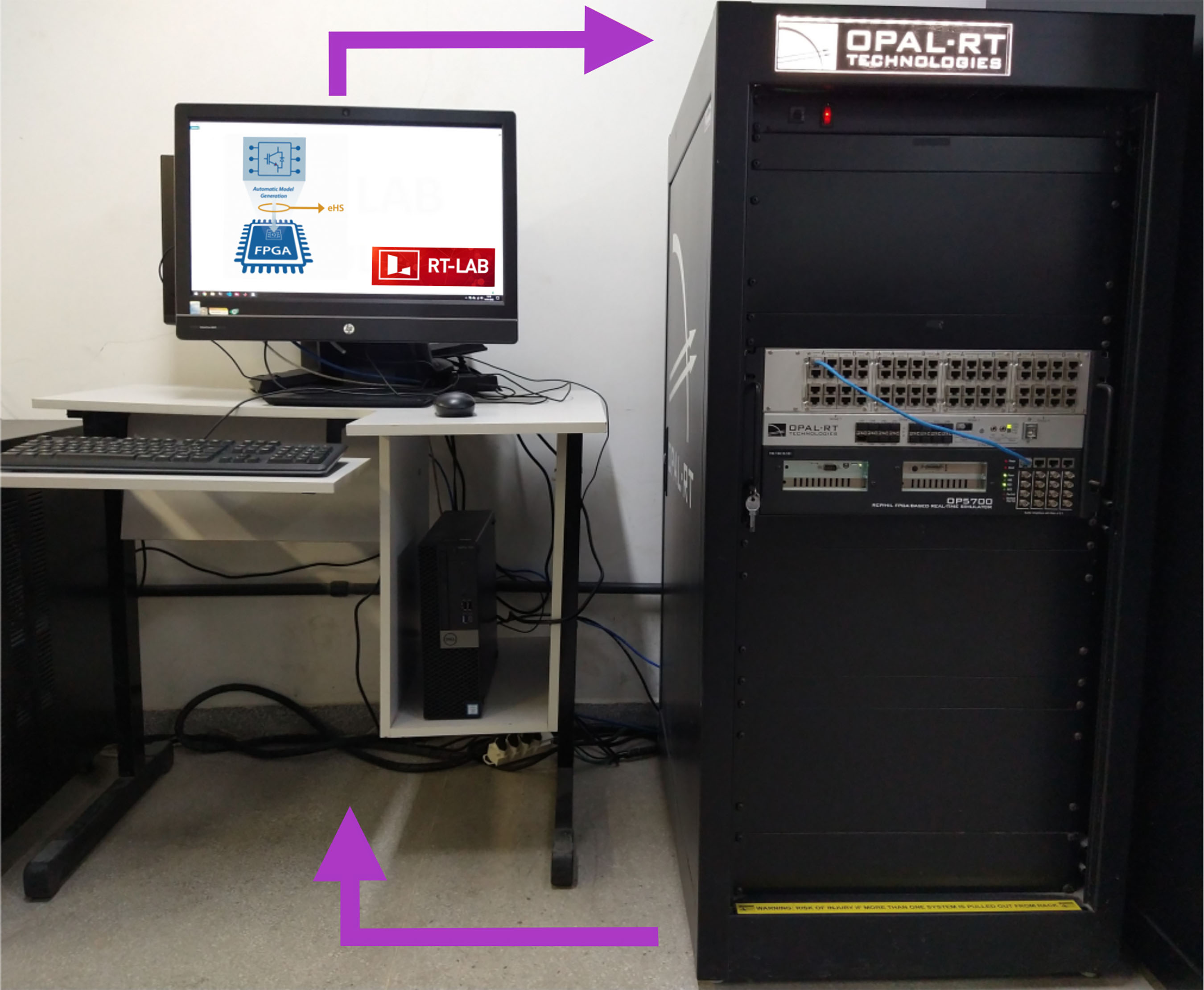
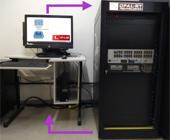
The results presented in this work were derived from realtime Model-in-the-Loop (MIL) simulations conducted using an OP5700 real-time simulator from OPAL-RT Technologies. The real-time simulation platform employed for validation is depicted in Figure 2.

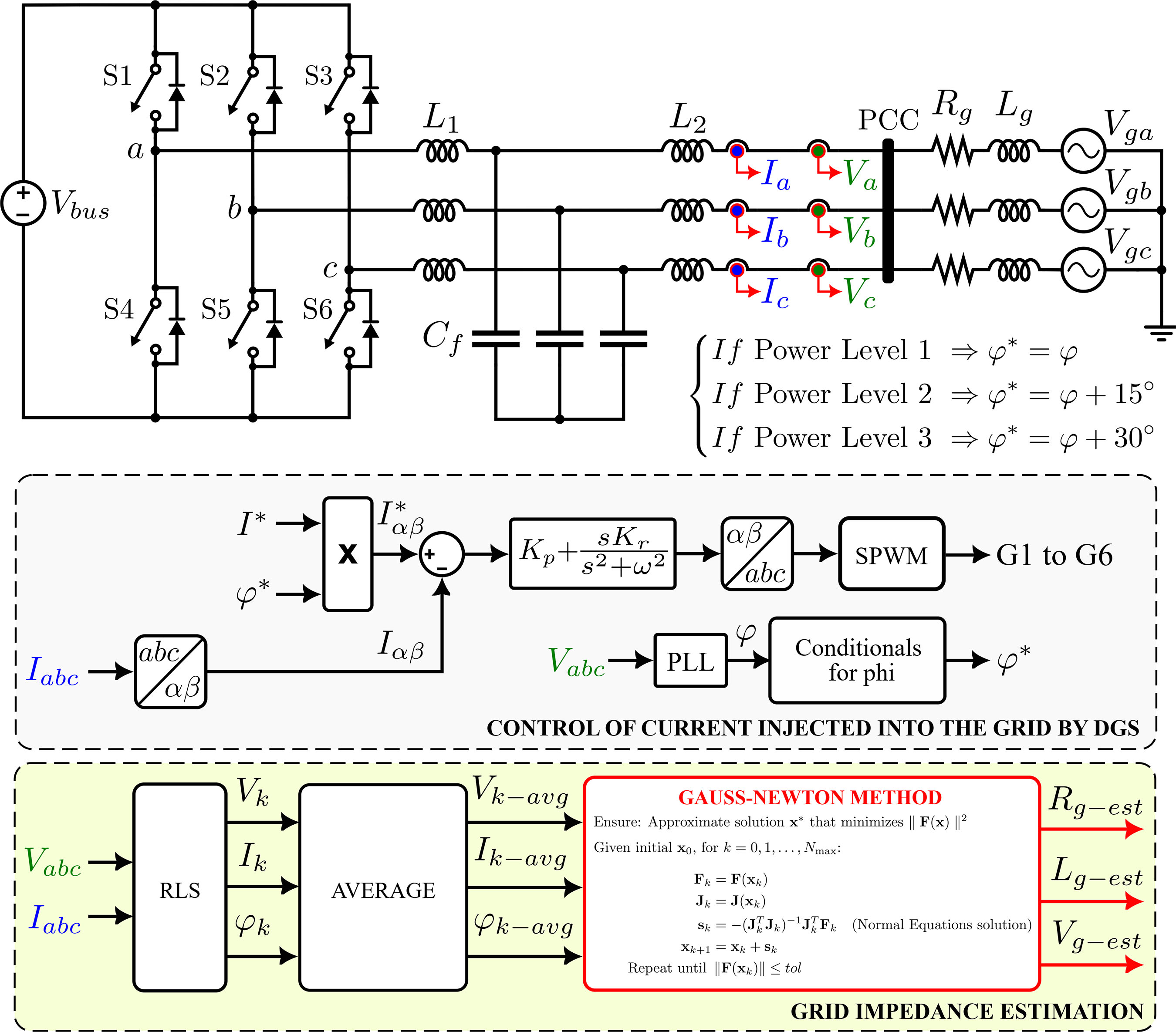
The complete system used for analysis is shown in Fig. 3. The system consists of a three-phase grid-connected inverter with an LCL output filter. The three operating points required to estimate the grid impedance are obtained by imposing different reference current levels (I^∗) and phase angles (φ^∗). All parameters used are presented in Table 2.

FIGURE 3
Complete schematic used to analyze the performance of the Gauss-Newton method.

TABLE 2
System parameters used for validation.

Parameter	Value
Grid Voltage (L-L)	230Vrms
Grid Frequency	50Hz
Grid Resistance	1 Ω
Grid Inductance	1mH
Active Power	1.8kW
K p	27
Kr	7000
L 1	20µH
L 2	0.5µH
C f	5µF
DC Link Voltage	400V
Switching Frequency	10kHz

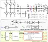
The values estimated by the recursive least squares (RLS) algorithm typically fluctuate around a nominal value. Consequently, a block denoted as Average was implemented, which computes the arithmetic mean of the last 12,500 samples contained within the final portion of the observation window (corresponding to the last 0.0125 s) for each of the three power levels. The resulting mean values of these segments of V_k, I_k, and φ_k are then provided as input to the block that implements the Gauss-Newton method.

It is important to observe that both the proposed and the traditional formulations provide an estimate of the inductive reactance X_g. Consequently, the corresponding inductance can be obtained by computing L_g = X_g/ω, where ω denotes the grid angular frequency, defined as ω = 2πf, with f representing the operating frequency.

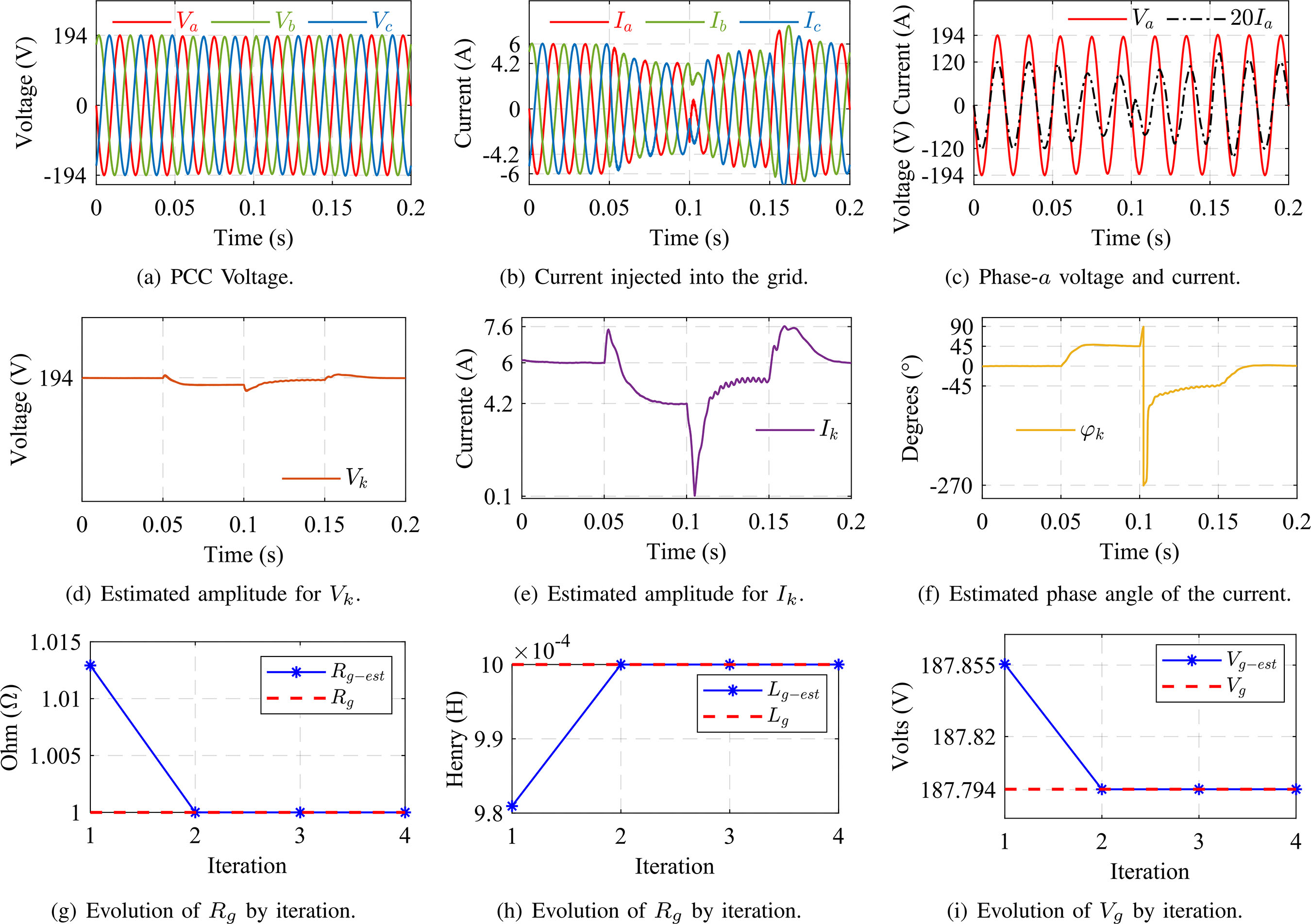
Fig. 4 contains the results obtained for the case when R_g = 1 and L_g = 1 mH. The first operating point goes from 0 to 0.05 s, the second from 0.05 to 0.1 s, and the third from 0.1 to 0.15 s. For the first level, a reference current equal to the nominal current was programmed; in the second, the reference current I^∗ is 70% of the nominal, and in the third operating point, 85% of the nominal. In (IV), the PCC voltage is shown during the estimation process. It can be noted that variations in the injected current have little impact on the PCC voltage, which is good, as it would not degrade the voltage profile delivered to possible local loads. Fig. (IV) shows the imposition of the control system on the current levels injected into the grid. In this, the duration and magnitude of each operating point are explicit. Fig. (IV) shows the phase difference between voltage and current for phase-a, as programmed in the first operating point, where voltage and current are in phase. In the second section, a delay (changing φ^∗) in the current of 45^◦ was programmed. In the last section, the current was advanced via the control system by 45^◦ about the voltage.

FIGURE 4
Results obtained for the case when R_g =1Ω and L_g =1 mH.

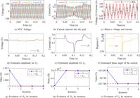
Figs. (IV), (IV) and (IV) show the efficiency of the RLS algorithm in estimating the amplitudes of the voltage at the PCC, the current injected into the grid, and the phase angle of this current, respectively. It is important to emphasize that the values used as input for the Gauss-Newton algorithm are collected after the transient seen at each change in the operating point has passed.

From Figs. (IV), (IV), and (IV) show the evolution of the estimated values at each iteration for R_g, L_g, and V_g, respectively. It was noted that all parameters were estimated with the appropriate predefined tolerance after four iterations.

Table 3 groups details of results obtained for different combinations of R_gL_g, including the case R_g = 1 Ω and L_g = 1 mH.

TABLE 3
Grid impedance estimation results for different cases.

Case	True Rg [Ω]	True Lg [mH]	Rg−est [Ω]	Lg−est [mH]	Rg Error [%]	Lg Error [%]	Exec. Time [ms]	Nº Iter.
1	0.0100	0.0100	0.0100	0.0099	0.0000	1.0000	0.3790	4
2	1.0000	1.0000	0.9956	1.0090	0.4400	0.9000	0.3630	4
3	5.0000	1.0000	4.9970	1.0200	0.0600	2.0000	0.3500	5
4	10.0000	0.5000	9.9900	0.4980	0.1000	0.4000	0.7460	5
5	0.5000	1.2000	0.4916	1.1730	1.6800	2.2500	0.7170	4
6	1.0000	1.5000	0.9926	1.5160	0.7400	1.0666	0.2280	4

All results presented in this work were obtained from the exact initial guess, which was 0.1 Ω, 0.1 Ω, and 180 V, for R_g, X_L, and V_g, respectively. In cases 1, 3, and 4, the resistance error is less than 0.1%. The inductance error did not exceed 2.25% in any of the cases discussed. The accuracy is remarkable even in cases with extreme impedance values, as in case 4 (with R_g = 10 Ω). These results indicate that the algorithm is robust and not overly sensitive to variations in the actual values of the parameters to be estimated.

In all cases, the number of iterations required for convergence varies between 4 and 5. This is a fundamental characteristic of the Gauss-Newton method, which, being a second-order method, tends to converge quadratically. The low number of iterations, in turn, contributes to a reduced runtime, less than 0.8 ms for all cases. Convergence speed is crucial for real-time estimation applications.

The inductance L_g acts as a filter, but it also impacts the dynamic response of the control system. When L_g is too large, the current rate of change di/dt becomes slower for a given voltage, meaning the inverter’s current controller needs more time to track the references. If the controller is not adjusted to compensate for this slower dynamic range, the control system’s phase margin decreases, leading to oscillations or even instability. Furthermore, the presence of a high grid inductance L_g, in conjunction with inverter output filters (such as LCL), can create low-frequency resonant poles that can be excited by noise or transients, making control and accurate current injection difficult. This occurred in cases 5 and 6, where the value of L_g is relatively high (1.2 mH and 1.5 mH, respectively). Therefore, the slightly larger percentage errors in these cases are not a flaw in the estimation algorithm itself, but rather a reflection of a larger inaccuracy in the input measurements, caused by the more challenging current injection dynamics imposed by the higher value of the grid inductance.

TABLE 4
Sensitivity of the Gauss-Newton method to initial conditions for true R_g =1Ω and L_g =1 mH.

Case	Vg0 [V]	Rg0 [Ω]	Lg0 [mH]	Rg−est [Ω]	Lg−est [mH]	Rg Error [%]	Lg Error [%]	Exec. Time [ms]	Nº Iter.
1	0.7 · Vg−nom	0.1	0.1	0.9913	1.0258	0.8700	2.5800	0.685	5
2	1.3 · Vg−nom	0.1	0.1	0.9927	1.0563	0.7300	5.6300	0.828	5
3	Vg−nom	0.01	0.01	0.9936	1.0084	0.6400	0.8400	0.322	4
4	Vg−nom	5.0	5.0	0.9962	1.0185	0.3800	1.8500	0.442	4
5	Vg−nom	20.0	10	0.9814	1.0365	1.8600	3.6500	0.483	6

To further assess the numerical stability of the proposed 3×3 formulation, a dedicated sensitivity analysis was performed, the results of which are summarized in Table 4. It should be noted that the results presented in Table 3 already provide an implicit evaluation of the method’s robustness, with x₀ held constant while the true parameters were varied; the algorithm successfully accommodated discrepancies up to 1,000 times the initial guess.

In Table 4, V_g-nom denotes the nominal grid voltage magnitude, V_g0 represents the initial guess for the grid voltage, and R_g0 and L_g0 correspond to the initial values assigned to the grid resistance and inductance, respectively, which are used to initialize the estimation procedure. This Table further investigates the sensitivity of the proposed method by systematically varying the initial voltage guess (V_g0) and imposing extreme deviations in the initial impedance values.

In Cases 1 and 2, the algorithm converges even in the presence of a ±30% error in V_g0, with a maximum error in the estimated L_g of 5.63%. Cases 3 to 5 show that choosing V_g0 equal to the nominal grid voltage yields estimation errors below 2% for both R_g and L_g, even when the initial impedance values range from 0.01× to 20× their true values. The computation time consistently remains below 1 ms, indicating that the reduced-order formulation is computationally efficient and robust against realistic levels of parameter uncertainty. Given that the nominal grid voltage is typically available, the recommended practice is to initialize the algorithm with V_g0 set equal to the nominal grid voltage.

V. CONCLUSION

This paper presents an optimized formulation for the grid impedance estimation problem. The approach consists of solving the problem in a 3x3 nonlinear system, which is significantly smaller than those currently reported in the literature. The system was formulated as a least-squares problem, which enabled the use of the Gauss-Newton method.

Despite the mathematical equivalence for quadratic systems, there are strong justifications for preferring the Gauss-Newton formulation in estimation problems, even when the number of equations and variables is the same. The Gauss-Newton method, by minimizing the sum of squares, tends to be more robust in the presence of slight noise in the measurements (which is common in real-world scenarios). This is because the method seeks the best fit rather than an exact root, which may not even exist due to the presence of noise.

It is very common for an initially square model to be later extended to include more measurements or incorporate redundancy to improve the robustness of the estimated parameters. Using the Gauss-Newton formulation facilitates this transition, as the algorithm’s structure (normal equations) is already prepared to handle non-square Jacobian matrices. When using the Newton-Raphson method in overdetermined systems, it is necessary to significantly refactor the algorithm to handle the non-square Jacobian, whereas Gauss-Newton already does so naturally.

To validate the proposal, real-time simulations were performed, implementing the proposed approach in the control system of a three-phase inverter with an LCL filter connected to the grid. The strategy employed consisted of imposing three operating points via the control system, estimating the voltage and current amplitudes at the PCC, as well as the current phase angle, and using these values as inputs to the 3x3 nonlinear system, making it solvable. It was noted that this strategy is highly dependent on the quality of the estimates of these quantities; however, the RLS algorithm proved to be robust enough for this type of application.

Six different combinations of R_gL_g were analyzed, and errors of less than 2.25% were observed in the estimates compared to the actual values. Furthermore, the Gauss-Newton algorithm’s execution time was less than 1 ms, requiring a worst-case scenario of 5 iterations to converge.

Based on the results obtained, it can be concluded that the proposed formulation is effective and provides significant benefits for increasing the robustness and computational efficiency of this type of system. Its use can make the online grid impedance estimation process faster and less computationally expensive.

ACKNOWLEDGMENT

The authors express their gratitude to the Coordination for the Improvement of Higher Education Personnel (CAPES), for their financial backing of this study.

• PLAGIARISM POLICY
  This article was submitted to the similarity system provided by Crossref and powered by iThenticate – Similarity Check.

DATA AVAILABILITY

The data used in this research is available in the body of the document.

REFERENCES

• ¹ International Energy Agency - IEA, “The Evolution of Energy Efficiency Policy to Support Clean Energy Transitions”, Digital Format, December 2023, URL: https://www.iea.org/reports/the-evolution-of-energyefficiency-policy-to-support-clean-energy-transitions
  » https://www.iea.org/reports/the-evolution-of-energyefficiency-policy-to-support-clean-energy-transitions
• ² T. B. Hadj, A. Ghodbane, E. B. Mohamed, A. A. Alfalih, “The transition to renewable energy through financial development and under natural resources threshold in emerging countries”, Environment, Development and Sustainability, Jan 2024, doi:10.1007/s10668-023-04389-1.
  » https://doi.org/10.1007/s10668-023-04389-1
• ³ F. Blaabjerg, Z. Chen, S. Kjaer, “Power electronics as efficient interface in dispersed power generation systems”, IEEE Transactions on Power Electronics, vol. 19, no. 5, pp. 1184–1194, 2004, doi:10.1109/TPEL.2004.833453.
  » https://doi.org/10.1109/TPEL.2004.833453
• ⁴ J. Sun, “Impedance-based stability criterion for grid-connected inverters”, IEEE Trans Power Electron, vol. 26, no. 11, pp. 3075–3078, Nov. 2011, doi:10.1109/TPEL.2011.2136439.
  » https://doi.org/10.1109/TPEL.2011.2136439
• ⁵ M. K. De Meerendre, E. Prieto-Araujo, K. H. Ahmed, O. Gomis-Bellmunt, L. Xu, A. Egea-Àlvarez, “Review of Local Network Impedance Estimation Techniques”, IEEE Access, vol. 8, pp. 213647–213661, 2020, doi:10.1109/ACCESS.2020.3040099.
  » https://doi.org/10.1109/ACCESS.2020.3040099
• ⁶ A. V. Timbus, P. Rodriguez, R. Teodorescu, M. Ciobotaru, “Line Impedance Estimation Using Active and Reactive Power Variations”, in 2007 IEEE Power Electronics Specialists Conference, pp. 1273–1279, 2007, doi:10.1109/PESC.2007.4342176.
  » https://doi.org/10.1109/PESC.2007.4342176
• ⁷ M. Cespedes, J. Sun, “Adaptive Control of Grid-Connected Inverters Based on Online Grid Impedance Measurements”, IEEE Transactions on Sustainable Energy, vol. 5, no. 2, pp. 516–523, 2014, doi:10.1109/TSTE.2013.2295201.
  » https://doi.org/10.1109/TSTE.2013.2295201
• ⁸ J. Sun, “Frequency-Domain Stability Criteria for Converter-Based Power Systems”, IEEE Open Journal of Power Electronics, vol. 3, pp. 222–254, 2022, doi:10.1109/OJPEL.2022.3155568.
  » https://doi.org/10.1109/OJPEL.2022.3155568
• ⁹ K. Pedersen, A. Nielsen, N. Poulsen, “Short-circuit impedance measurement”, IEE Proceedings - Generation, Transmission and Distribution, vol. 150, pp. 169–174, 2003, doi:10.1049/ipgtd:20030193.
  » https://doi.org/10.1049/ipgtd:20030193
• ¹⁰ S. Cobreces, E. J. Bueno, D. Pizarro, F. J. Rodriguez, F. Huerta, “Grid Impedance Monitoring System for Distributed Power Generation Electronic Interfaces”, IEEE Transactions on Instrumentation and Measurement, vol. 58, no. 9, pp. 3112–3121, 2009, doi:10.1109/TIM.2009.2016883.
  » https://doi.org/10.1109/TIM.2009.2016883
• ¹¹ N. Mohammed, T. Kerekes, M. Ciobotaru, “An Online Event-Based Grid Impedance Estimation Technique Using Grid-Connected Inverters”, IEEE Transactions on Power Electronics, vol. 36, no. 5, pp. 6106–6117, 2021, doi:10.1109/TPEL.2020.3029872.
  » https://doi.org/10.1109/TPEL.2020.3029872
• ¹² D. O. Cardoso, H. M. T. C. Gomes, F. A. d. C. Bahia, A. P. N. Tahim, J. R. Pinheiro, F. F. Costa, “Impacto do PLL para Estimação de Impedância de Rede e Avaliação de Estabilidade no Domínio DQ em Sistemas com Inversores Conectados”, Eletrônica de Potência, vol. 28, no. 2, p. 107–118, Mar. 2023, doi:10.18618/REP.2023.2.0050.
  » https://doi.org/10.18618/REP.2023.2.0050
• ¹³ Y. Cheng, W. Wu, Y. Yang, E. Koutroulis, H. S.-H. Chung, M. Liserre, F. Blaabjerg, “Zero-Sequence Voltage InjectionBased Grid Impedance Estimation Method for Three-Phase Four-Wire DC/AC Grid-Connected Inverter”, IEEE Transactions on Industrial Electronics, vol. 71, no. 7, pp. 7273–7279, 2024, doi:10.1109/TIE.2023.3306395.
  » https://doi.org/10.1109/TIE.2023.3306395
• ¹⁴ J. Mace, A. Cervone, D. Dujic, “Self-Synchronized Grid Impedance Estimation Unit Using Interpolated DFT Technique”, IEEE Transactions on Power Electronics, vol. 39, no. 4, pp. 4624–4635, 2024, doi:10.1109/TPEL.2023.3342317.
  » https://doi.org/10.1109/TPEL.2023.3342317
• ¹⁵ J. Fang, H. Deng, S. M. Goetz, “Grid Impedance Estimation Through Grid-Forming Power Converters”, IEEE Transactions on Power Electronics, vol. 36, no. 2, pp. 2094–2104, 2021, doi:10.1109/TPEL.2020.3010874.
  » https://doi.org/10.1109/TPEL.2020.3010874
• ¹⁶ H. M. T. C. Gomes, L. L. O. Carralero, J. H. Suárez, A. P. N. Tahim, J. R. Pinheiro, F. F. Costa, “Estimativa de Impedância para Suporte de Estabilidade e Qualidade de Energia em Inversores Conectados à Rede”, Eletrônica de Potência, vol. 27, no. 2, p. 165–176, Jun. 2022, doi:10.18618/REP.2022.2.0004.
  » https://doi.org/10.18618/REP.2022.2.0004
• ¹⁷ H. M. T. C. Gomes, L. L. O. Carralero, J. H. Suárez, A. N. Tahim, J. R. Pinheiro, F. F. Costa, “A Grid Impedance Estimation Method Robust Against Grid Voltages Unbalance and Harmonic Distortions”, Journal of Control, Automation and Electrical Systems, vol. 34, no. 2, pp. 289–301, apr 2023, doi:10.1007/s40313-022-00963-6.
  » https://doi.org/10.1007/s40313-022-00963-6
• ¹⁸ J. R. P. de Assis, A. d. S. Gomes, H. M. T. C. Gomes, F. F. Costa, W. F. Felipe, M. B. d. R. Corrêa, D. A. Fernandes, “Iterative Methods for Nonlinear Systems Applied to Grid Impedance Estimation: A Comparative Study”, Eletrônica de Potência, vol. 29, p. e202446, Nov. 2024, doi:10.18618/REP.e202446.
  » https://doi.org/10.18618/REP.e202446
• ¹⁹ D. A. Fernandes, S. R. Naidu, C. Coura, “Instantaneous Sequence-Component Resolution of 3-Phase Variables and Its Application to Dynamic Voltage Restoration”, IEEE Transactions on Instrumentation and Measurement, vol. 58, no. 8, pp. 2580–2587, 2009, doi:10.1109/TIM.2009.2015634.
  » https://doi.org/10.1109/TIM.2009.2015634
• ²⁰ I. Argyros, Computational Theory of Iterative Methods, vol. 15, Elsevier Science, 2007.

Edited by

• Associate Editor
  Roberto F. Coelho https://orcid.org/0000-0002-4672-0885

• Editor-in-Chief
  Allan F. Cupertino https://orcid.org/0000-0001-8418-1985

Publication Dates

• Publication in this collection
  06 July 2026
• Date of issue
  2026

History

• Received
  11 Feb 2026
• Reviewed
  03 Apr 2026
• Accepted
  06 Apr 2026
• Published
  08 May 2026