Obstacle Avoidance Control of Multi-Parafoil Formation Based on Spatial Velocity Vector Method

ABSTRACT

The obstacle avoidance flight of unmanned parafoil formations in complex terrains and under wind disturbances is essential for the success of airdrop missions. This study develops a comprehensive dynamic model of the parafoil and constructs a three-dimensional mountainous simulation environment. An obstacle avoidance algorithm based on the spatial velocity vector method is proposed, which dynamically regulates the parafoil’s motion through traction, avoidance, and guidance velocity vectors, thereby achieving efficient obstacle avoidance in complex wind fields. By incorporating a consensus-based leader-follower formation control strategy, the parafoil formation maintains both geometric configuration and heading stability during obstacle avoidance maneuvers. Simulation results demonstrate that the proposed method effectively enables safe obstacle avoidance and stable formation flight under wind disturbances, confirming the effectiveness of the algorithm.

Keywords
Parafoils; Formation flying; Automatic flight control; Obstacle avoidance; Wind velocity

INTRODUCTION

Unmanned parafoil vehicles (UPVs), also known as controllable or ram-air parafoils, can perform maneuverable flight and precise fixed-point landings by adjusting the trailing-edge control lines. Compared with conventional round parachutes, UPVs exhibit greater controllability and enhanced resistance to wind disturbances. They possess broad application potential in areas such as the airdrop of earthquake-relief materials and battlefield logistics resupply. Consequently, UPVs have increasingly attracted the attention of academia and industry. Compared with conventional unmanned aerial vehicles (UAVs), parafoil-based unmanned systems offer advantages such as high payload capacity, low operational cost, and superior flexibility, making them suitable for deployment in a wide range of complex environments (Sun et al. 2024).

In recent years, research on parafoils has primarily focused on a single-parafoil system, yielding substantial achievements. Zhou et al. (2024) propose a three-dimensional trajectory-tracking control method based on a bilinear active disturbance rejection control strategy. This method is developed for the six-degree-of-freedom parafoil model and achieves attitude and position trajectory tracking through the coordinated design of guidance laws and control algorithms. Li et al. (2024b) investigate trajectory planning for the parafoil system using an original natural algorithm, incorporating digital representations of external environmental factors such as wind fields and terrain. The study successfully validates the algorithm’s rationality and demonstrates its advantages in terms of efficiency and safety. Wang and Yang (2024) perform numerical simulations of the aerodynamic characteristics of parafoils using the lattice Boltzmann method. The results verify the reliability of the method and reveal that incorporating a curved canopy significantly enhances the lift-drag characteristics, while the internal cell structure plays a crucial role in improving overall performance. These studies provide valuable reference and guidance for parafoil testing and simulation, thereby laying a solid foundation for future research on multi-parafoil formation systems.

In practical missions such as earthquake-relief and battlefield supply airdrops, it is often necessary to deploy multiple parafoils simultaneously to fulfill mission requirements. Consequently, the need for research on multi-parafoil formation airdrops has become increasingly pressing. During large-scale precision airdrop and fixed-point landing missions, parafoils frequently encounter complex and dynamic obstacles, including highland terrain, mountainous regions, enemy defenses, and urban structures. To ensure mission success, the flight dynamics and obstacle avoidance capabilities of parafoil formations must be comprehensively considered. Given that parafoils possess limited control authority and lack propulsion systems, multiple constraints-including obstacle avoidance, yaw angle, and glide path-must be jointly considered to ensure the feasibility of obstacle avoidance control.

While ensuring the feasibility of flight trajectories, it is essential to enhance the cooperative dynamic obstacle avoidance capability of multi-parafoil formations so that formation members can effectively respond to diverse challenges and operational demands in complex environments. In recent years, extensive research has focused on obstacle avoidance strategies for aerial formations. Zhang et al. (2024) introduce multi-agent deep reinforcement learning and multi-agent proximal policy optimization, leveraging digital twin technology to overcome sampling limitations and resource constraints, and develop an architecture for training UAV formation obstacle avoidance models. Huang et al. (2024) propose an obstacle avoidance control strategy for wingman formations based on the deep deterministic policy gradient algorithm, integrating the artificial potential field (APF) method with leader-follower consensus control. Zhao et al. (2024) develop motion, perception, and communication models between UAVs and ground robots, design a coordinated motion-control framework, and propose a dynamic formation-boundary generation method encompassing shape control, collision avoidance, formation keeping, and navigation control, thereby achieving self-regulating formations. Addressing the multi-UAV obstacle avoidance problem in constrained environments is essential for enhancing UAV safety and mission efficiency, and it remains a central research focus in this field.

The design of a robust, safe, and highly flexible obstacle avoidance algorithm for parafoil formations represents a challenging yet significant research endeavor. Each parafoil within the formation must autonomously avoid external obstacles while preventing inter-parafoil collisions; hence, it is necessary to concurrently manage both external obstacles and internal spatial relationships among formation members. This necessitates the integration of existing algorithms with parafoil dynamic models and the implementation of algorithmic design within a three-dimensional simulation environment.

Problem description

The obstacle avoidance problem of multi-parafoil formation systems primarily concerns the overall motion of the system. Attitude variations of the parafoil system and the relative motions among internal components, such as the canopy and payload, are not the primary factors considered in formation obstacle avoidance (Zhao et al. 2022). Therefore, a kinematic model of the parafoil system is sufficient to satisfy the requirements of this study.

Parafoil point-mass model

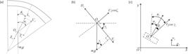
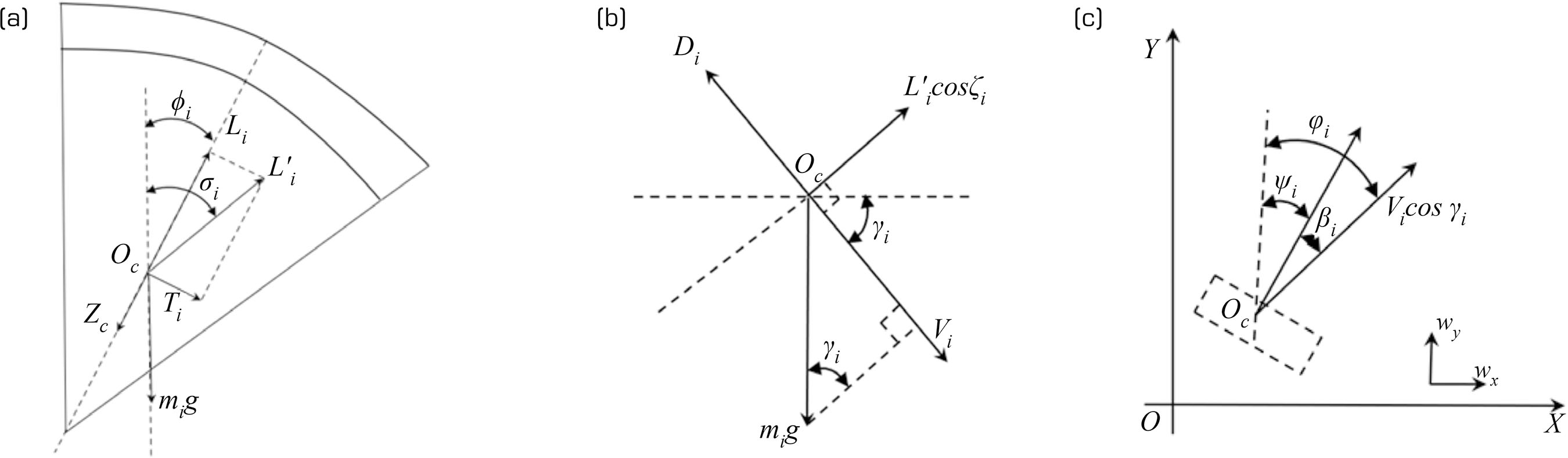
As shown in Fig. 1, the schematic diagram illustrates the forces acting on the parafoil system. In the parafoil formation, the main forces include the aerodynamic lift L_i generated by the canopy, the lateral force T caused by the canopy’s inclination, and the resultant aerodynamic force L_i′ , which is the vector sum of the lift and the lateral force. Due to the influence of the lateral force, the actual lift L_i′ cos σ_i produced by the system is perpendicular to the velocity vector V_i , while σ_i represents the angle between the resultant aerodynamic force and the vertical direction. φ_i denotes the inclination angle of the parafoil system, and the flight-path angle γ_i is defined as the angle between the parafoil trajectory and the horizontal plane. ψ_i represents the yaw angle, ϕ_i the heading angle, and β_i the sideslip angle. During free glide, β_i = 0 , and therefore ϕ_i = ψ_i. In the inertial coordinate system, w_x and w_y represent the components of the wind velocity along the x-axis and y-axis, respectively.

Figure 1
Schematic diagram of the parafoil system. (a) Rear view; (b) Side view; (c) Top view.

Based on the above analysis, the parafoil can be described by the following differential equations:

(1) $\{\begin{array}{l}{\dot{x}}_i=V_i\cos {\gamma }_i\cos {\phi }_i+w_x,\\ {\dot{y}}_i=V_i\cos {\gamma }_i\sin {\phi }_i+w_y,\\ {\dot{z}}_i=V_i\sin {\gamma }_i,\end{array}$

(2) $\{\begin{array}{l}{\dot{V}}_i=-\frac{m_{i}g\sin {\gamma }_i+D_i}{m_i},\\ {\dot{\gamma }}_i=\frac{L_i^{\prime }\cos {\zeta }_i-m_{i}g\cos {\gamma }_i}{m_i{V}_i},\\ {\dot{\phi }}_i=\frac{L_i^{\prime }\sin {\zeta }_i}{m_i{V}_i\cos {\gamma }_i},\end{array}$

where i = 0,1, 2,..., N , (x_i, y_i, z_i) denotes the position of the parafoil system in the Earth-fixed coordinate system, V_i represents the total airspeed of the parafoil, ϕ_i denotes the yaw angle, and γ represents the glide (flight-path) angle, w_x and w_y represent the components of the environmental wind velocity along the x- and y-axes in the Earth-fixed coordinate system, mi denotes the mass of the -th parafoil, D_i represents the aerodynamic drag, L'_i denotes the resultant lift, and ζ_i represents the roll (bank) angle of the parafoil system, which depends on the differential deflection of the left and right trailing-edge control lines. By differentiating Eq. 1 and substituting Eq. 2 into the resulting expression, the second-order point-mass model of the parafoil system is derived as follows:

(3) $\{\begin{array}{l}\dot{\mathit{p}}={\mathit{v}}_i,\\ {\dot{\mathit{v}}}_i={\mathit{u}}_i,\end{array}$

where ${\mathit{p}}_i={[x_i,y_i,z_i]}^T$ denotes the position vector of the -th parafoil in the formation, ${\mathit{v}}_i={[V_{xi},V_{yi},V_{zi}]}^T$ represents its velocity vector, and ${\mathit{u}}_i={[U_{xi},U_{yi},U_{zi}]}^T$ denotes the equivalent control-input vector of the -th parafoil along the three axes of the Earth-fixed coordinate frame. After determining the equivalent control variable u_i, the bank (tilt) angle of the parafoil system can be computed using the following expression:

(4) ${\varphi }_i={\tan }^{-1}\left(\frac{U_{yi}\cos {\chi }_i-U_{xi}\sin {\chi }_i}{\cos {\gamma }_i(U_{zi}+\mathrm{g})-\sin {\gamma }_i(U_{xi}\cos {\chi }_i+U_{yi}\sin {\chi }_i)}\right).$

Under steady-state conditions, the motion of the parafoil system can be decomposed into uniform horizontal and vertical components. The glide ratio of k the parafoil system is defined as follows:

(5) $k=\frac{V_{xy}}{V_z}=\frac{\sqrt{{\dot{x}}^2+{\dot{y}}^2}}{\dot{z}},$

Accordingly, the glide angle can be expressed as follows:

(6) $\gamma =\arctan \left(\frac{1}{k}\right).$

Therefore, under steady-state conditions, the trajectory of the parafoil system forms a curve characterized by a constant glide angle. The parafoil primarily controls its heading through adjustments of the trailing-edge control lines, resulting in flight characteristics that differ from those of fixed-wing aircraft. Accordingly, constraints are imposed on the maximum allowable variations of the heading and glide angles at each time step. The motion-performance constraints of the parafoil system are therefore defined as follows:

(7) $\mathrm{\Delta }\phi =|{\phi }_{i+1}-{\phi }_i|\le \mathrm{\Delta }{\phi }_{max},\mathrm{\forall }i=0,1,\dots$

(8) $\mathrm{\Delta }\gamma =|{\gamma }_{i+1}-{\gamma }_i|\le \mathrm{\Delta }{\gamma }_{max},\mathrm{\forall }i=0,1,\dots ,$

The above expressions indicate that the variations in the parafoil’s yaw and glide angles between two consecutive time steps do not exceed their prescribed maximum limits.

Mountain environment model

Based on the operational requirements of parafoil airdrop missions, a mountainous-terrain simulation environment is constructed. Without loss of generality, enemy air-defense systems can likewise be modeled as mountainous obstacles within the simulation to represent complex terrain conditions (Chen et al. 2019).

$h(x,y)=h_0+\sum _{i=1}^n{h}_i\cdot \exp [-{\left(\frac{x-x_{0i}}{x_{si}}\right)}^2-{\left(\frac{y-y_{0i}}{y_{si}}\right)}^2],$

In Eq. 9, h₀ denotes the reference terrain elevation, h_i represents the maximum elevation of the -th mountain peak, x_0i and y_0i denote the coordinates of the peak point of the -th mountain, x_si and y_si and correspond to slope-related parameters of the -th mountain along the - and -axes, respectively.

Spatial velocity vector algorithm

Basic principles

The fundamental concept of the spatial velocity vector method is to abstract the entire planning space into a velocity-vector field (Ren 2023), where the target point and obstacle regions act as field sources. Each point within the field corresponds uniquely to a velocity vector that specifies both magnitude and direction. The corresponding definitions are presented as follows:

• Field source: the origin that generates the velocity field, encompassing the target point and threat (obstacle) regions.

• Field strength: the velocity magnitude and direction induced at a planning point by the field source.

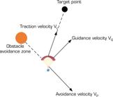
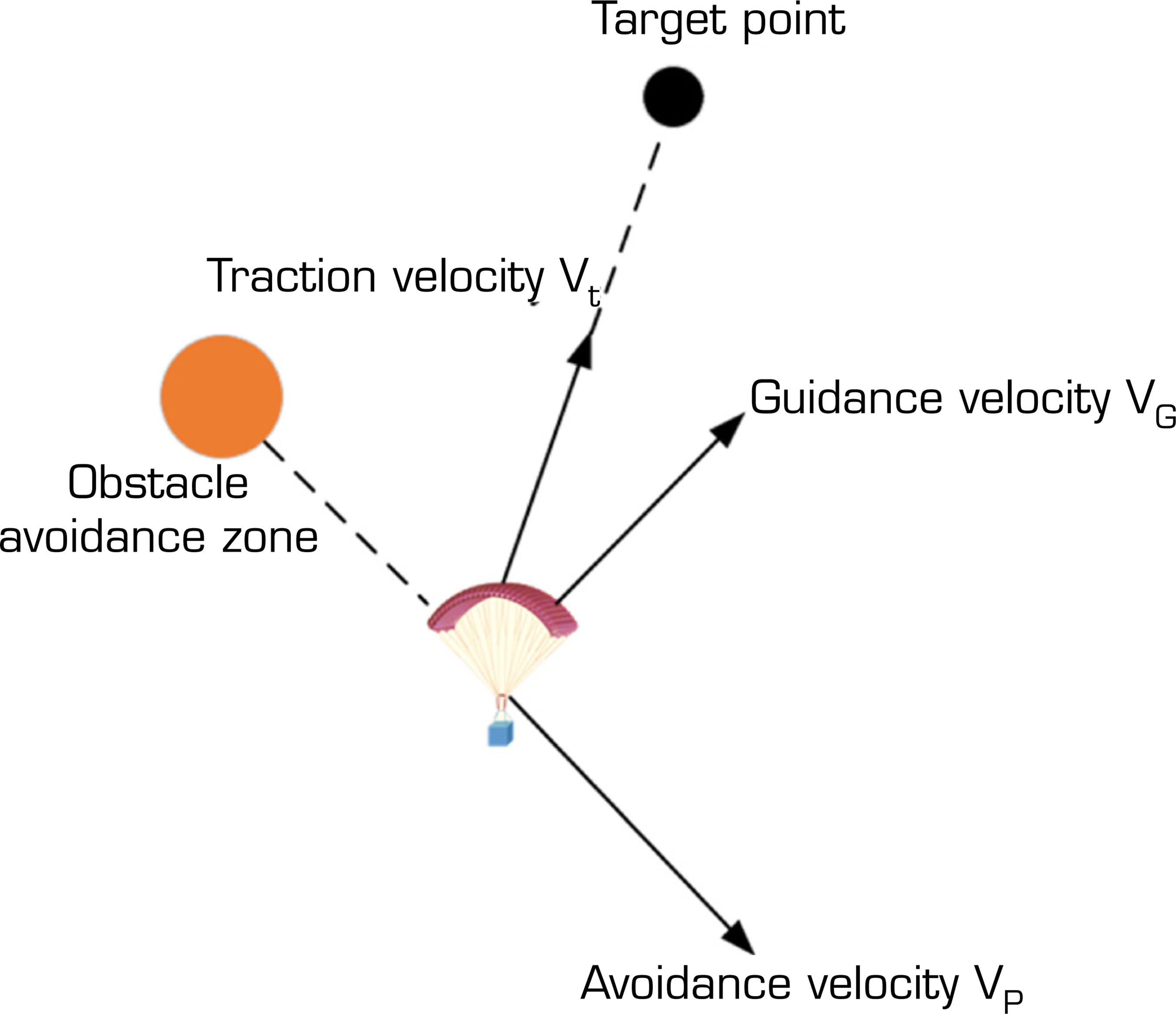
In the formation obstacle avoidance algorithm based on the spatial velocity-vector method, the target point acts as the source of the traction field, generating a traction velocity. The obstacle regions act as the sources of both the avoidance and guidance fields, generating not only an avoidance velocity but also a guidance velocity that is orthogonal to the avoidance component and directed toward the target point. A schematic illustration of the field relationships is shown in Fig. 2.

Figure 2
Schematic diagram of spatial velocity vector.

The spatial velocity-vector method was developed on the basis of the APF approach. The APF approach offers advantages such as simple implementation, low computational complexity, and strong real-time performance, and it has been widely employed in UAV real-time obstacle avoidance tasks. However, the APF approach is prone to becoming trapped in local minima, particularly when the repulsive and attractive forces reach equilibrium, which prevents the UAV from continuing to move toward the target.

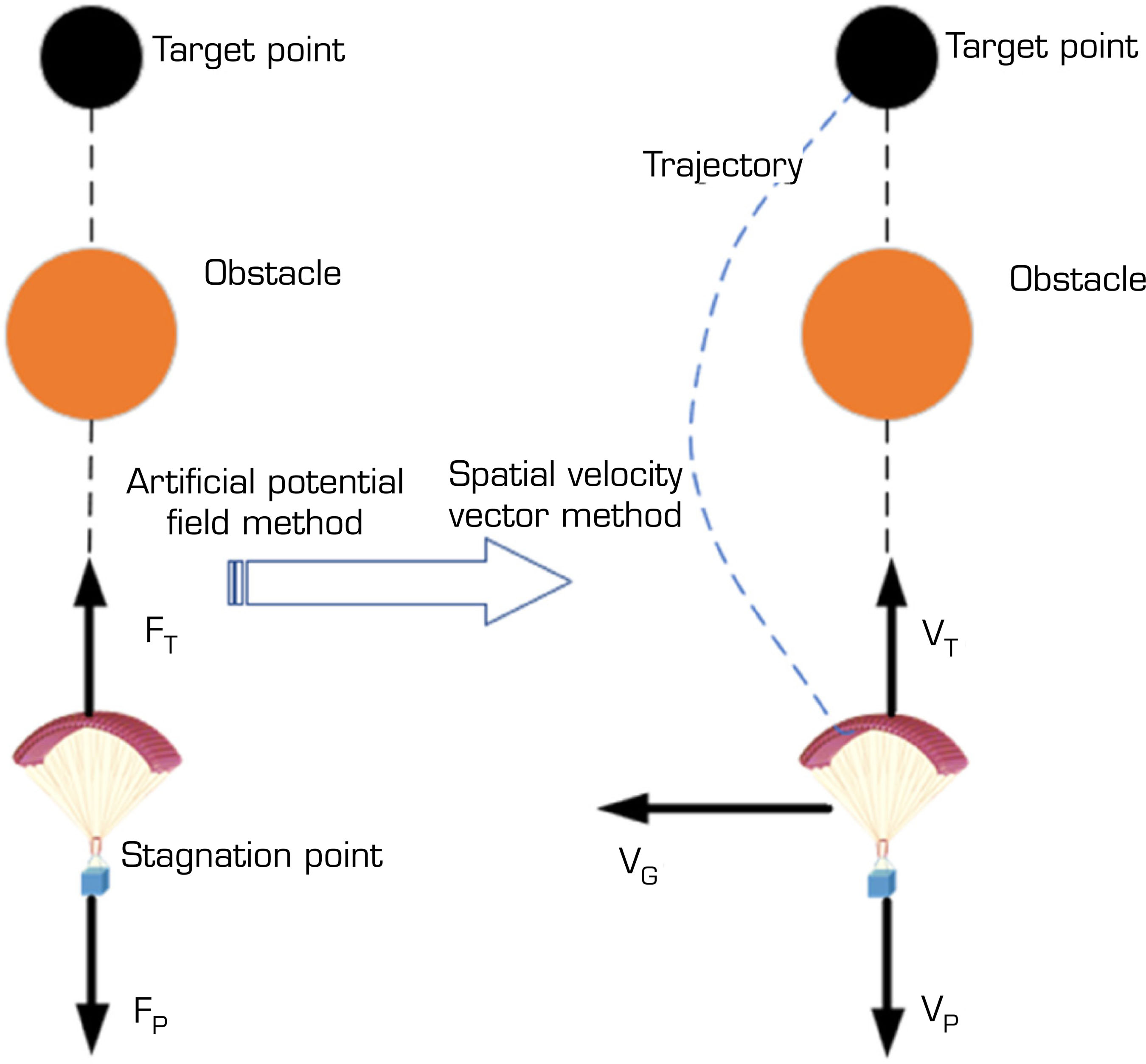
As illustrated in Fig. 3, when the parafoil is positioned at the stagnation point, the APF approach exhibits a local minimum. At this point, the attractive force F_T generated by the target and the repulsive force F_P exerted by the obstacle become balanced, causing the planning point to lose propulsion and remain stationary. In contrast, within the spatial velocity-vector field method, the presence of the guidance velocity ensures that the resultant velocity remains nonzero, allowing the parafoil to continue advancing toward the target point.

Figure 3
Improved local minimum problem.

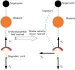
At the stagnation point, the traction velocity V_T and the avoidance velocity V_P cancel each other out, yielding V_T + V_P = 0. The total resultant velocity V in the spatial velocity vector method is the sum of three components: V = V_T + V_P + V_G. Substituting the stagnation condition simplifies this to V = V_G. Because the guidance velocity is V_G perpendicular to V_P, and V_P ≠ 0 within the influence range of the obstacle, the magnitude of V_G is also not zero. Consequently, the resultant velocity V_P ≠ 0, providing a lateral motion to actively push the parafoil out of the equilibrium state.

The principal advantage of the spatial velocity-vector method lies in the fact that the resultant quantity acting on the controlled object is a resultant velocity rather than a resultant force, effectively abstracting the notion of mass and thereby enhancing both responsiveness and maneuverability. In addition, the introduction of the guidance velocity helps to eliminate the mutual constraints between the traction velocity and the avoidance velocity, thereby significantly alleviating the local-minimum problem inherent in the APF approach.

Traction velocity

Throughout the entire flight process of the parafoil, the traction influence exerted by the target point must persist (Gao and Tao 2022). Its direction is defined from the current position of the parafoil toward the target point. The functional expression of the traction velocity V_T is defined as follows:

(10) ${\mathit{V}}_T=\omega \cdot {\mathit{r}}_t,$

In Eq. 10, the vector V_T denotes the target traction velocity, ω represents the weighting coefficient of the traction field, and r_t denotes the unit direction vector of the traction velocity, whose expression r_t is given as follows:

(11) $\{\begin{array}{l}{r}_{tx}=\frac{x_c-x_t}{\sqrt{{(x_c-x_t)}^2+{(y_c-y_t)}^2}},\\ r_{ty}=\frac{y_c-y_t}{\sqrt{{(x_c-x_t)}^2+{(y_c-y_t)}^2}},\end{array}$

In Eq. 11, r_tx denotes the x-axis component of the vector r_t, r_ty denotes the y-axis component of the vector r_t, (x_c, y_c) represents the current position coordinate vector, and (x_t, y_t) represents the coordinate vector of the target point.

Avoidance velocity

The obstacle region acts as the source of the avoidance field, generating an avoidance velocity V_P that directs the current trajectory point away from nearby obstacles. A buffer zone is defined around each obstacle, within which the field strength of the avoidance field varies gradually to ensure smooth repulsive transitions (Zheng et al. 2023).

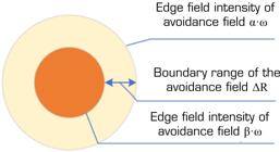
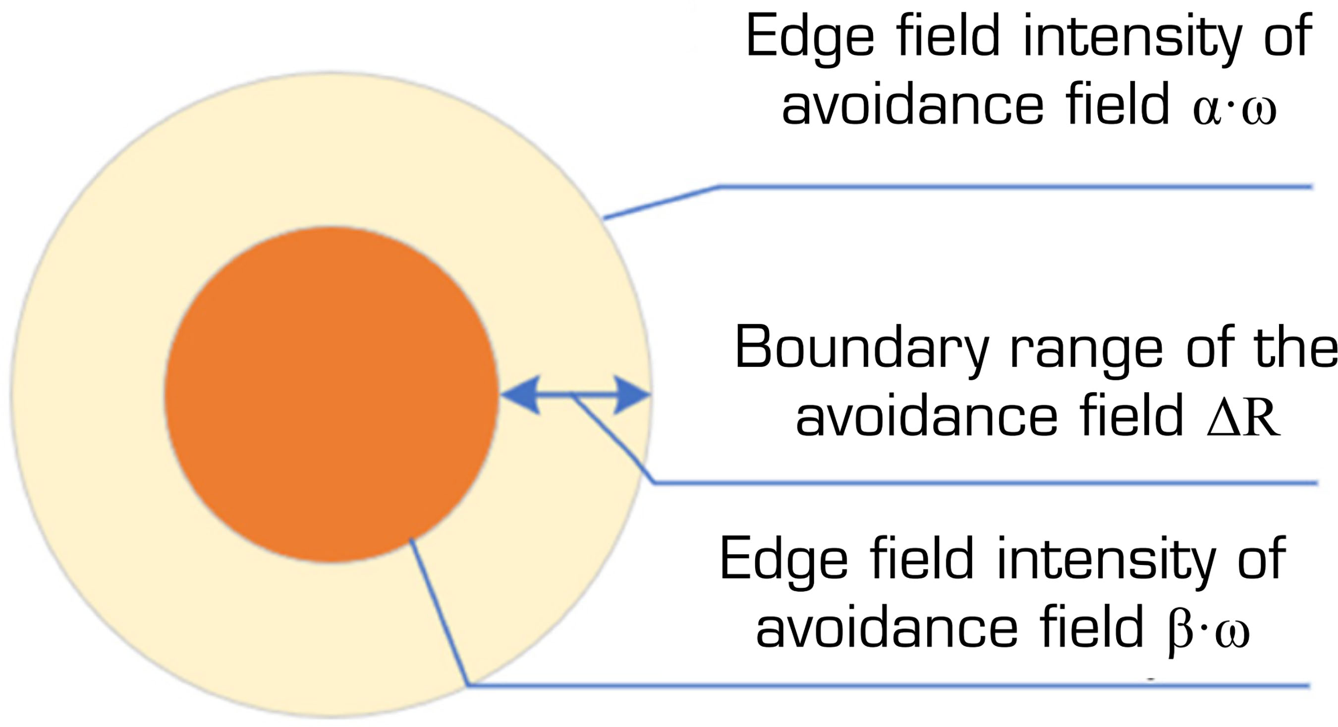
As illustrated in the schematic diagram of the avoidance-field model, the effective influence range of the obstacle region is denoted by ∆R. The maximum and minimum field strengths of the obstacle region are denoted by β·ω and α·ω, respectively. As the distance between the parafoil and the obstacle region increases, the avoidance-field strength decreases gradually, following an inverse-square relationship with respect to distance. When the distance exceeds the threshold ∆R, the parafoil is no longer influenced by the field strength of that obstacle region (Qin et al. 2018). The calculation formula for the avoidance-field strength is given as follows:

(12) ${\mathit{V}}_p^i=\{\begin{array}{ll}0,& d_i>r_i+\mathrm{\Delta }R,\\ \frac{{\omega }_p}{1+{((d_i-r_i)/L)}^2}\cdot r_p^i,& r_i\le d_i\le r_i+\mathrm{\Delta }R,\\ \frac{{\omega }_p}{{(d_i/r_i)}^2}\cdot r_p^i,& d_i<r_i,\end{array}$

In Eq. 12, Vⁱ_pdenotes the avoidance velocity induced by the -th obstacle at the current position of the parafoil, ω_p represents the weighting coefficient of the avoidance field, L denotes the influence coefficient of the avoidance field, d_i represents the distance between the current parafoil position and the center of the -th obstacle, r_i denotes the radius of the -th obstacle, ∆R denotes the effective influence range of the avoidance field, and rⁱ_p represents the unit direction vector of the avoidance velocity induced by the -th obstacle (Li et al. 2024a), as expressed below:

(13) $\{\begin{array}{l}{r}_{px}^i=\frac{x_c-x_o^i}{\sqrt{{(x_c-x_o^i)}^2+{(y_c-y_o^i)}^2}},\\ r_{py}^i=\frac{y_c-y_o^i}{\sqrt{{(x_c-x_o^i)}^2+{(y_c-y_o^i)}^2}},\end{array}$

In Eq. 13, ${\mathit{r}}_{px}^i$ denotes the x-axis component of the vector rⁱ_p and ${\mathit{r}}_{py}^i$ denotes the y-axis component of the vector rⁱ_p, (x_c, y_c) represents the coordinate vector of the current position, and (xⁱ_o, yⁱ_o) represents the coordinate vector of the -th obstacle’s center. The value of w_p is determined by parameters β and the weighting coefficient ω of the traction field, while the value of L is determined by parameters α, β, and R, as expressed below (Li et al. 2021):

(14) ${\omega }_p=\beta \cdot \omega ,$

(15) $L=\frac{\mathrm{\Delta }R}{\sqrt{\beta /\alpha }}$

As indicated by the above equation, the magnitude of the avoidance velocity V_P is solely determined by parameters α, β, and ΔR.

Guidance velocity

When the parafoil encounters mountainous obstacles during its gliding flight, a guidance velocity is introduced in addition to the avoidance velocity induced by the terrain, assisting the parafoil in moving away from the obstacle (Sun et al. 2022). The incorporation of the guidance velocity provides directional bias during obstacle avoidance, enabling the parafoil to escape from local-minimum conditions.

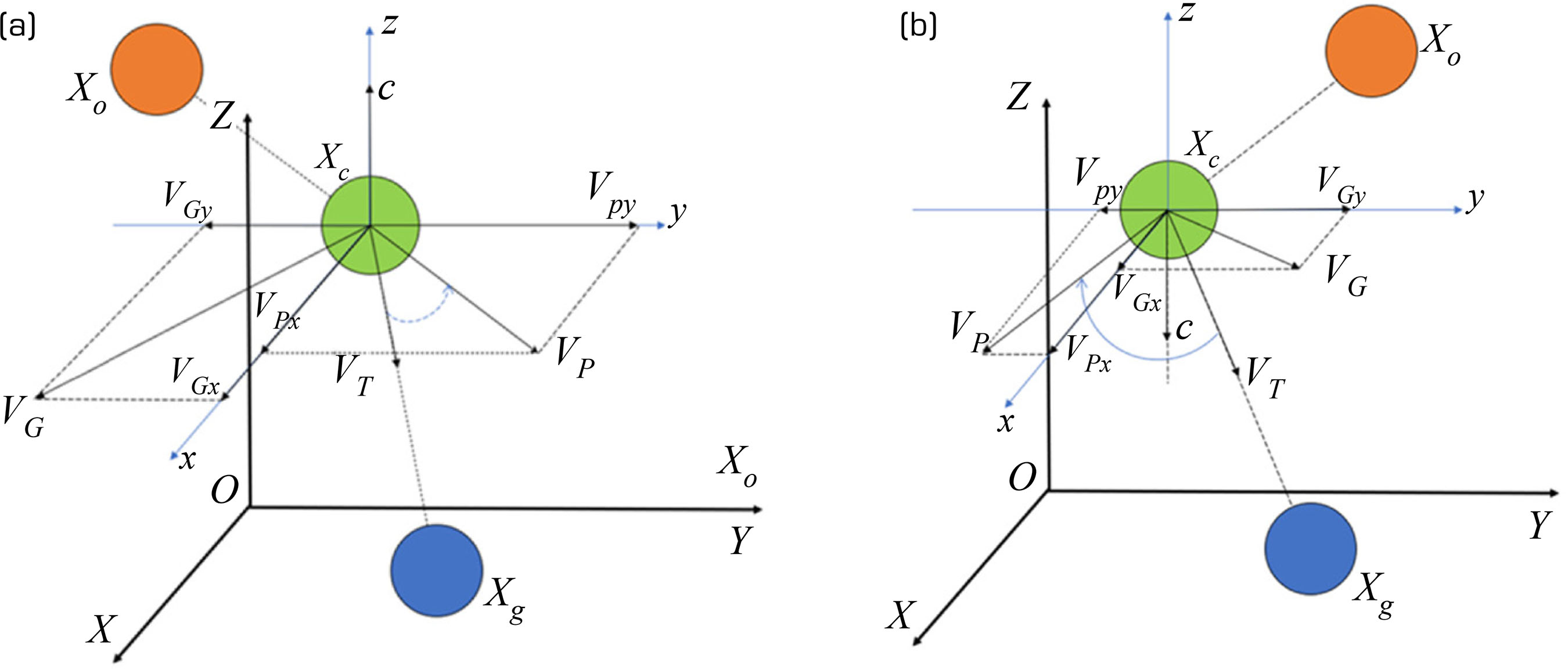
The guidance velocity is generated within mountainous obstacle regions and is produced concurrently with the avoidance velocity. First, the vector cross product (a, b, c)^T = V_T × V_P between the traction velocity V_T and the avoidance velocity V_P is defined. The corresponding calculation formulas for a, b, and c are given as follows (Zhao et al. 2023):

(16) $(a,b,c)=(r_{ty}{r}_{pz}-r_{tz}{r}_{py},r_{tz}{r}_{px}-r_{tx}{r}_{pz},r_{tx}{r}_{py}-r_{px}{r}_{ty})$

The direction of the guidance velocity V_G is orthogonal to the avoidance velocity and oriented toward the target direction. Depending on the sign of the parameter c, the computation of the guidance velocity V_G can be divided into two cases, which are derived from the geometric relationships illustrated in Fig. 4. Based on the value of c, the rotation direction is determined according to the right-hand rule. In the coordinate system, the arrow indicates the positive orientation of the coordinate axes. By projecting the avoidance velocity V_P onto the x- and y-axes (Lu et al. 2022), the corresponding components V_Px and V_Py are obtained. According to Eq. 13, the guidance velocity V_G can then be calculated from the avoidance velocity V_P. In Fig. 5a and b, orange spheres denote obstacles, the green sphere indicates the current parafoil position, and the blue sphere corresponds to the target point in the obstacle avoidance algorithm. It can be observed that, under the influence of the guidance velocity, the parafoil gradually deflects toward the target direction while avoiding obstacles.

Figure 4
Schematic diagram of the avoidance field.

Figure 5
Schematic diagram of guidance velocity calculation. (a) Case of ; (b) Case of .

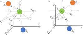
The calculation formula of the guidance velocity is given as follows:

(17) $\{\begin{array}{ll}(V_{Gx},V_{Gy})=(\epsilon V_{P_y},-\epsilon V_{P_x})& c>0,\\ (V_{Gx},V_{Gy})=(-\epsilon V_{Py},\epsilon V_{Px})& c\le 0,\end{array}$

In the above equation, V_Gx and V_Gy denote the x- and y-axis components of the guidance velocity, respectively, V_px and V_py denote the x- and y-axis components of the avoidance velocity, respectively, and ε represents the ratio between the field strengths of the guidance and avoidance fields (Jia et al. 2024). In this study, the parameter ε is set to 1, indicating that the field strengths of the guidance and avoidance fields are considered equal. This specific value is chosen to strike an optimal dynamic balance between the efficiency of escaping a local minimum and the safety margin of obstacle avoidance. Specifically, if ε is set significantly higher than 1 (ε >> 1), the guidance velocity dominates, commanding an overly rapid lateral turning maneuver. While this allows for a quick escape from the stagnation point, the dominant guidance field may overpower the repulsive avoidance field, causing the trajectory to cut corners and risk penetrating the physical safety boundary of the obstacle. Conversely, if ε is set significantly lower than 1 (ε << 1) the repulsive avoidance field dominates, rendering the generated guidance velocity too weak to effectively push the parafoil laterally. As a result, the trajectory would exhibit sluggish lateral movement, prolonged stagnation, or even severe numerical oscillations, failing to bypass the obstacle efficiently. Therefore, setting ε = 1 ensures a smooth and timely escape trajectory while strictly respecting the safety clearance of the obstacles.

Parafoil formation design

In a consensus-based formation, the main challenge lies in how to apply consensus theory to model the parafoil formation as a network topology. By employing a consensus algorithm, the position, velocity, and other state variables of each parafoil can be synchronized with the predefined reference states. Furthermore, a distributed control structure within a leader-follower formation framework is adopted to realize coordinated formation control.

Formation control involves two coordination variables, namely, the position and velocity of each parafoil (Lu et al. 2024). If both conditions, $\underset{t\to \mathrm{\infty }}{lim}\left({\mathit{x}}_i\right(t)-{\mathit{x}}_j(t\left)\right)={\mathit{h}}_{ij}$ and $\underset{t\to \mathrm{\infty }}{lim}\left({\mathit{v}}_i\right(t)-{\mathit{v}}_d(t\left)\right)=0$, are satisfied, the formation can be successfully established and maintained. ${\mathit{x}}_i\left(t\right),{\mathit{x}}_j\left(t\right),{\mathit{v}}_i\left(t\right),\mathrm{and}{\mathit{v}}_d\left(t\right)$ denote the position vector, velocity vector, and desired velocity vector of individuals i and j, respectively, and h_y is determined by the formation geometry and denotes the desired relative distance vector between individuals i and j.

During the formation process, formation reconfiguration can be achieved by adjusting the formation vector, while formation speed regulation can be realized by modifying the desired velocity. Assuming that the desired formation vector and the formation motion velocity are known, the individual formation control law is designed as follows:

(18) ${\mathit{u}}_i\left(t\right)={\mathit{u}}_{i-form}\left(t\right)+{\mathit{u}}_{i-vel}\left(t\right)+{\mathit{u}}_{i-obs}\left(t\right)$

(19) ${\mathit{u}}_{i-form}\left(t\right)=-\sum _{j=1}^N{g}_{ij}{w}_{ij}\left({\mathit{x}}_i\right(t)-{\mathit{x}}_j(t)-{\mathit{h}}_{ij}),$

(20) ${\mathit{u}}_{i-1-vl}\left(t\right)={\dot{v}}_d\left(t\right)-\lambda \left(v_i\right(t)-v_d(t\left)\right)-\eta \sum _{j=1}^N{g}_{ij}{w}_{ij}\left(v_i\right(t)-v_j(t\left)\right),$

(21) $V_i=V_T+V_P+V_G,$

(22) ${\mathit{u}}_{i-abs}\left(t\right)={\mathit{V}}_i+{\rho }_0\sum _{k\in OBS}{P}_{i,k}\left({\mathit{x}}_i\right(t)-{\mathit{x}}_{obs,k}(t\left)\right),$

(23) $P_{i,k}=\frac{200}{\exp {\left(\frac{\left|{\mathit{x}}_i\right(t)-{\mathit{x}}_{obs,k}(t\left)\right|}{13.5}\right)}^{1.5}},$

In the above equation, u_i(t) represents the control vector of an individual parafoil in the formation, ${\mathit{v}}_d\left(t\right)={\mathit{v}}_d+{\dot{\mathit{v}}}_{d}t$ represents the formation control dynamics, where ${\dot{\mathit{v}}}_d\text{and}{\mathit{v}}_d$ denote the desired formation acceleration and the velocity, respectively, g_ij describes the communication topology, when information flows from parafoil i to parafoil j, g_ij = 1, otherwise is 0, w_ij > 0 represents the communication weight coefficient, λ > 0 , η > 0 , and N denote the total number of parafoils within the formation. Other parafoils in the formation are treated as dynamic obstacles relative to the current parafoil. ρ₀ denotes the weight coefficient of collision-avoidance control, P_i,k is a nonlinear function that increases as the current parafoil approaches other parafoils, x_i(t) denotes the position of the parafoil at time, x_{obs, k}(t) denotes the position of parafoil k, which is regarded as an obstacle, at the same time , and V_i represents the resultant potential-field input of the current parafoil.

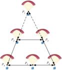
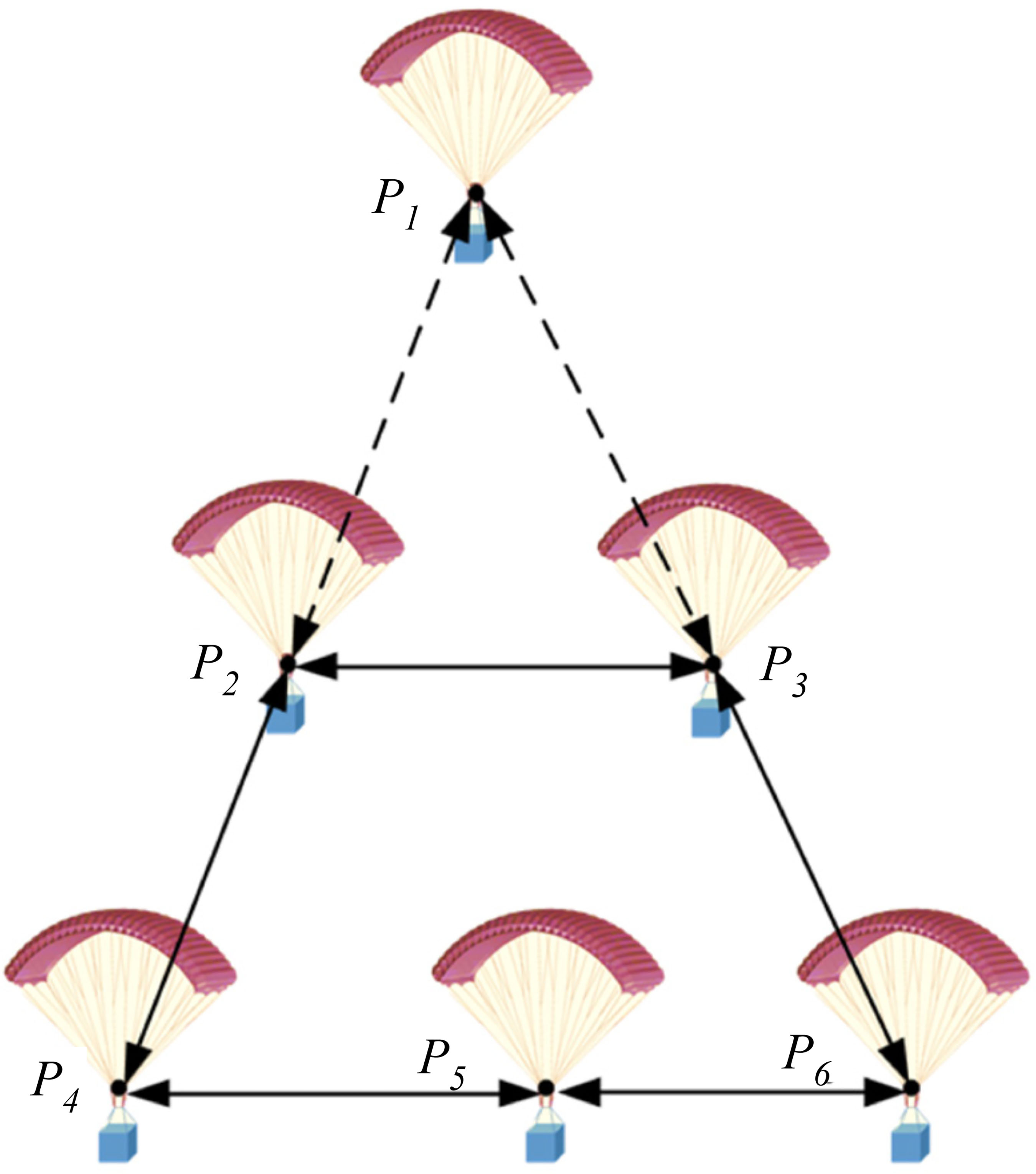
Throughout the formation process, the communication network topology (Ma et al. 2024) remains fixed, as illustrated in Fig. 6. In the topology, P₀ represents the leader parafoil, while the others are follower parafoils. As depicted in the figure, not all follower parafoils are required to receive information directly from the leader; only a subset needs to do so. In addition, follower parafoils communicate through bidirectional links, indicating that the follower topology constitutes an undirected graph. Each parafoil exchanges information only with its neighboring parafoils, without requiring access to global information from the entire formation. This local-information-based communication strategy effectively reduces wireless communication load and lowers the likelihood of nodes being detected by wireless reconnaissance. Beyond these benefits of communication, this specific topology offers distinct physical advantages. It avoids the high-frequency updates typical of fully connected networks, thereby providing a smooth reference trajectory suitable for the slow responding parafoil actuators. Additionally, these localized connections help maintain spatial separation, reducing the risk of aerodynamic wake vortex interference among the parafoils.

Figure 6
Communication topology of the multi-parafoil formation.

Stability analysis of the parafoil formation

The stability of the system is analyzed as follows:

(24) $$x=1$$

By integrating all control inputs of the parafoils, the overall system equation can be expressed as above, where denotes the Laplacian matrix of the system, whose elements characterize the interactions among different parafoils within the formation. denotes the number of parafoils in the formation, is associated with the desired formation configuration, and the specific definitions of the parameters are provided as follows:

(25) $\mathit{L}=\left[l_{ij}\right]={[{\mathit{L}}_1^T,{\mathit{L}}_2^T,\cdots ,{\mathit{L}}_N^T]}^T,$

(26) $I_{ij}=\{\begin{array}{ll}\sum _{j\ne j}{g}_{ij}{w}_{ij},& i=j,\\ -g_{ij}{w}_{ij},& i\ne j,\end{array}$

(27) ${\mathit{L}}_i=[l_{i1},l_{i2},\cdots l_{iN}]$

(28) $\mathit{E}=-{[h_1^1{L}_1^T,h_1^2{L}_1^T,\cdots ,h_1^n{L}_1^T,h_2^1{L}_2^T,\cdots ,h_N^n{L}_N^T]}^T.$

Based on Eqs. 1 and 16, the closed-loop system’s state equation is obtained after algebraic manipulation.

(29) $\dot{\epsilon }\left(t\right)=A\epsilon \left(t\right)+B,$

where

(30) $\mathit{A}=\left[\begin{array}{cc}0& {\mathit{I}}_{nN}\\ -(\mathit{L}\otimes {\mathit{I}}_n)& -\eta (\mathit{L}\otimes {\mathit{I}}_n)-\lambda {\mathit{I}}_{n\mathrm{N}}\end{array}\right],$

(31) $\mathit{B}=\left[\begin{array}{c}0\\ \mathit{E}+\lambda ({\mathit{l}}_N\otimes {\mathit{v}}_d)+{\mathit{l}}_N\otimes {\dot{\mathit{v}}}_d\end{array}\right].$

A and B denote the coefficient matrix and the bias vector of the closed-loop system, respectively. From the above equation, it can be observed that the matrix is a Laplacian matrix, which is symmetric and semipositive definite, with eigenvalues greater than or equal to zero. Since λ > 0 and η > 0 satisfy the given conditions, the damping matrix $\eta (\mathit{L}\otimes {\mathit{I}}_n)+\lambda {\mathit{I}}_{nN}$, constructed from the lower-triangular components, is strictly positive definite. According to the structural properties of the second-order system, all eigenvalues of matrix A have negative real parts, indicating that the system is asymptotically stable.

(32) $\mathit{\epsilon }\left(t\right)={\left[\begin{array}{ll}{\mathit{x}}^T\left(t\right)& {\mathit{v}}^T\left(t\right)\end{array}\right]}^T,$

where

(33) $x\left(t\right)={\left[\begin{array}{llll}{\mathit{x}}_1^T\left(t\right)& {\mathit{x}}_2^T\left(t\right)& \cdots & {\mathit{x}}_N^T\left(t\right)\end{array}\right]}^T,$

(34) $v\left(t\right)={\left[\begin{array}{llll}{\mathit{v}}_1^T\left(t\right)& {\mathit{v}}_2^T\left(t\right)& \cdots & {\mathit{v}}_N^T\left(t\right)\end{array}\right]}^T,$

where x(t) and v(t) denote the position and velocity vectors of the closed-loop system, respectively.

Simulation analysis

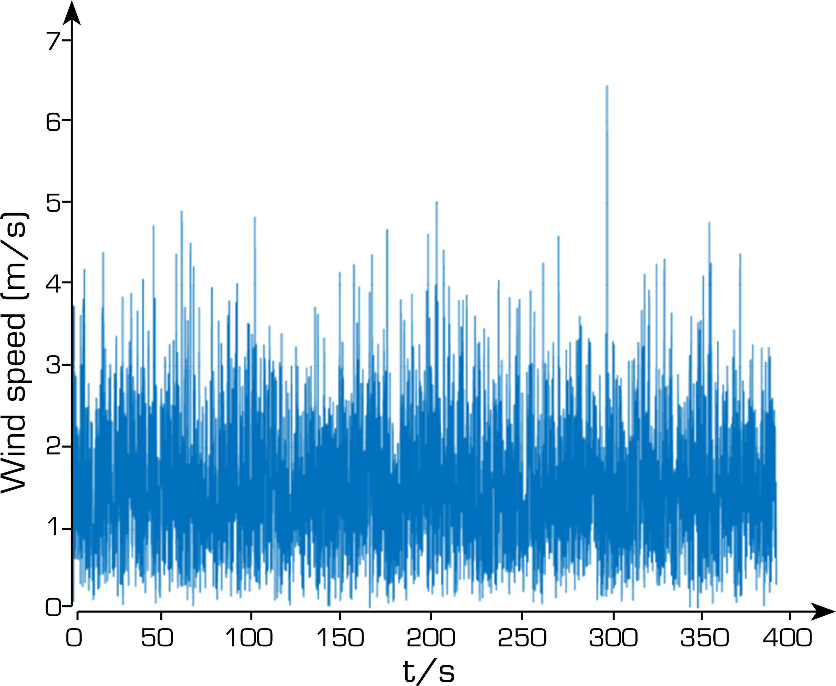
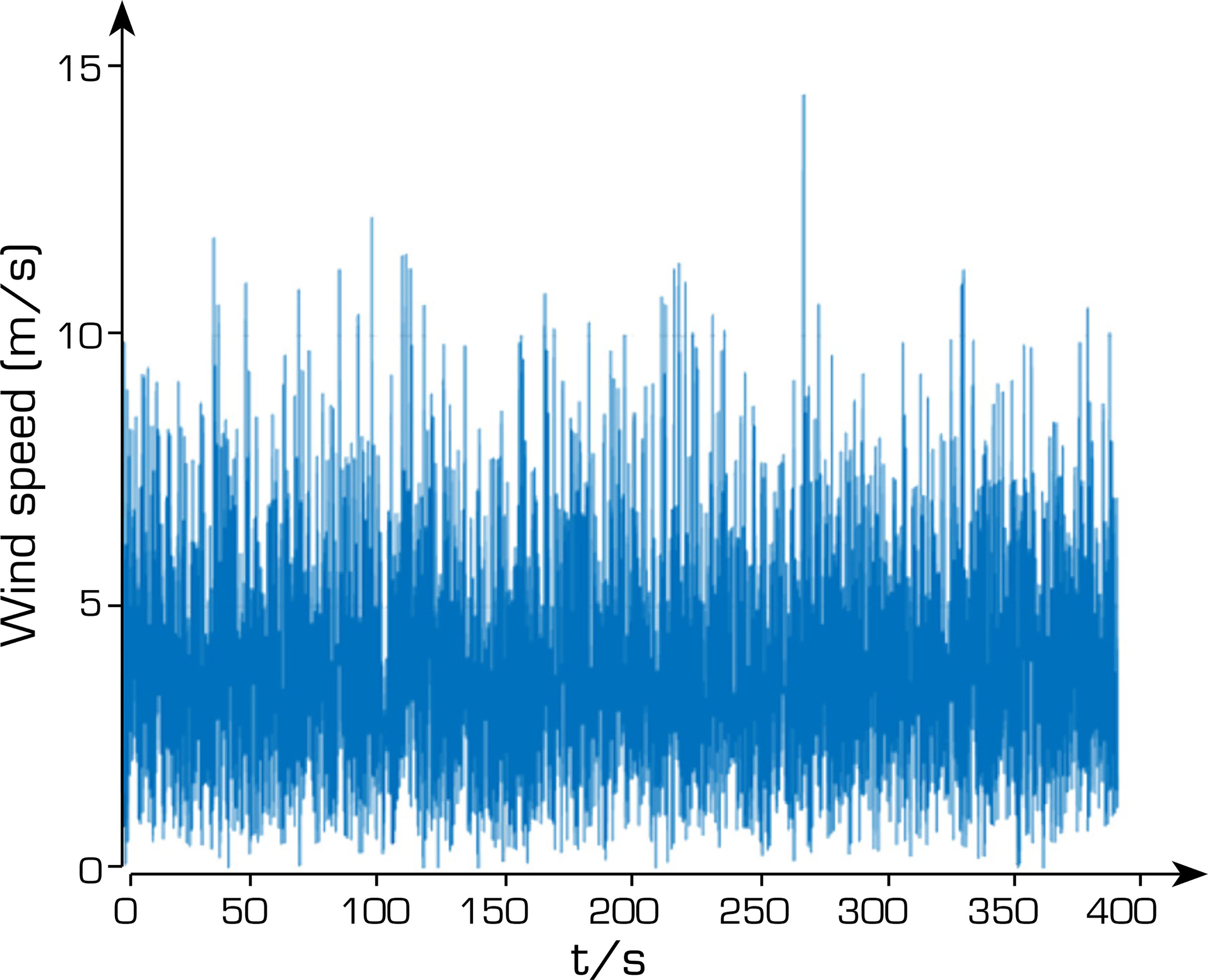
To verify the effectiveness of the formation obstacle avoidance algorithm proposed in this paper, a formation consisting of multiple parafoils is simulated to perform a fixed-point airdrop under mission scenarios involving multiple mountains. Horizontal random wind disturbances were introduced. Small gusts were modeled using random wind speeds primarily distributed around 2 m·s^-1, while large gusts were modeled with random wind speeds mainly concentrated around 5 m·s^-1. The parameters of the spatial velocity model employed in the simulations are configured accordingly, as summarized in Table 1. In the theoretical simulation, an allowable arrival radius of 1 m is utilized to verify the convergence and accuracy of the algorithm. Considering environmental disturbances and sensor errors in practical missions, this arrival condition is typically relaxed to a more realistic radius (e.g., 20 m to 30 m), depending on the system scale.

Table 1
Simulation parameters.

Parameter	Value
Target point	(0, 0, 0)
Initial position of parafoil 1	(1500, 600, 2000)
Initial position of parafoil 2	(1800, 900, 2000)
Initial position of parafoil 3	(2100, 800, 2000)
Initial position of parafoil 4	(800, 1300, 2000)
Initial position of parafoil 5	(600, 1500, 2000)
Initial position of parafoil 6	(500, 1900, 2000)
α	0.02
β	0.9
ΔR	200
ε	1

• Source: Elaborated by the authors.

Formation obstacle avoidance of parafoils in multi-mountain terrain

This simulation case is conducted to verify the validity of the spatial velocity model, specifically to examine whether the three velocity components V_T, V_P, and V_G of the parafoil achieve the intended traction and avoidance effects, and whether the selected field-strength parameters α, β, and ∆R are appropriately chosen.

The simulation scenario involves three mountains of varying locations and heights to construct the obstacle avoidance environment for the parafoils. A formation composed of six parafoils is simulated to perform an airdrop mission.

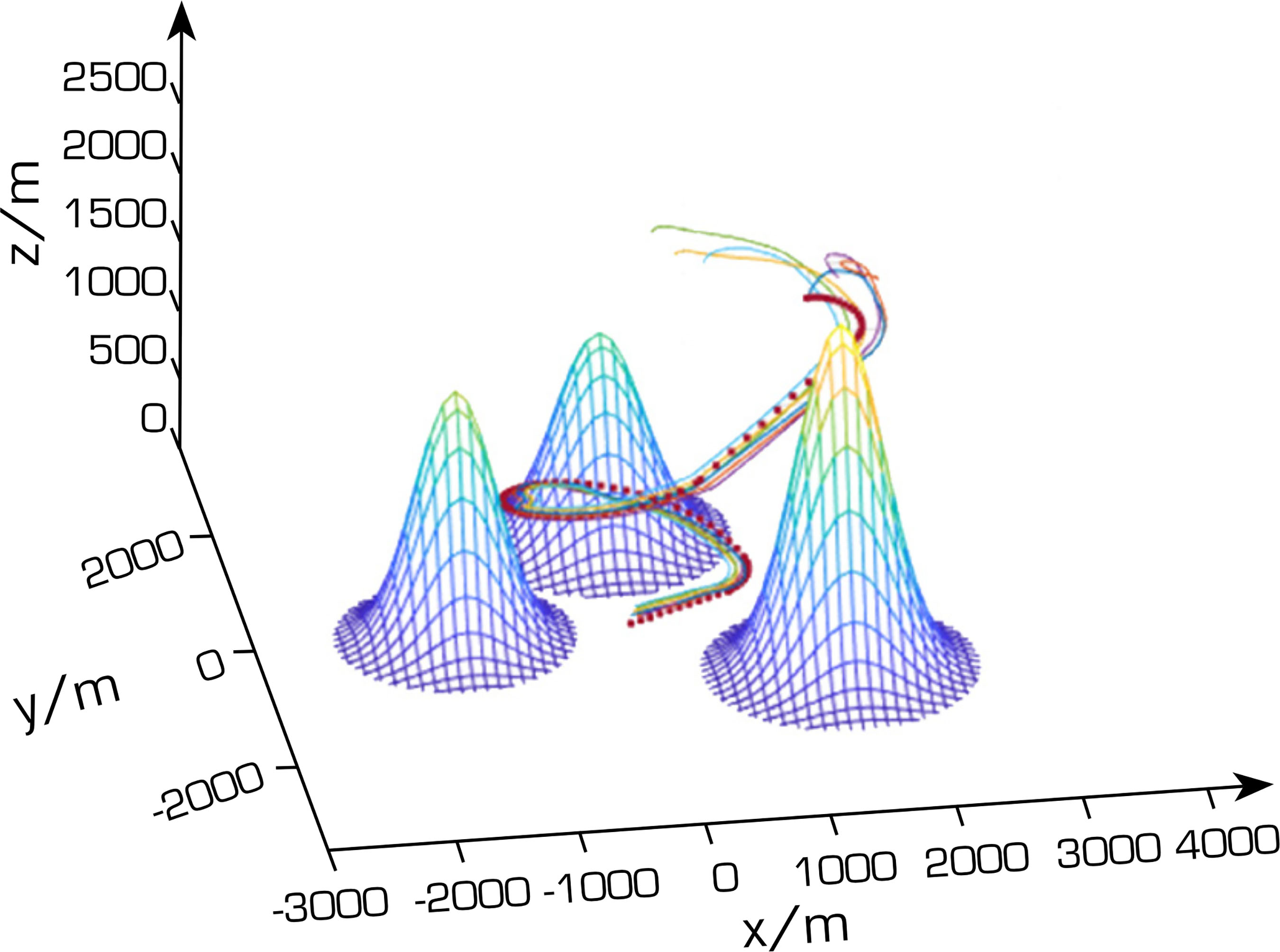
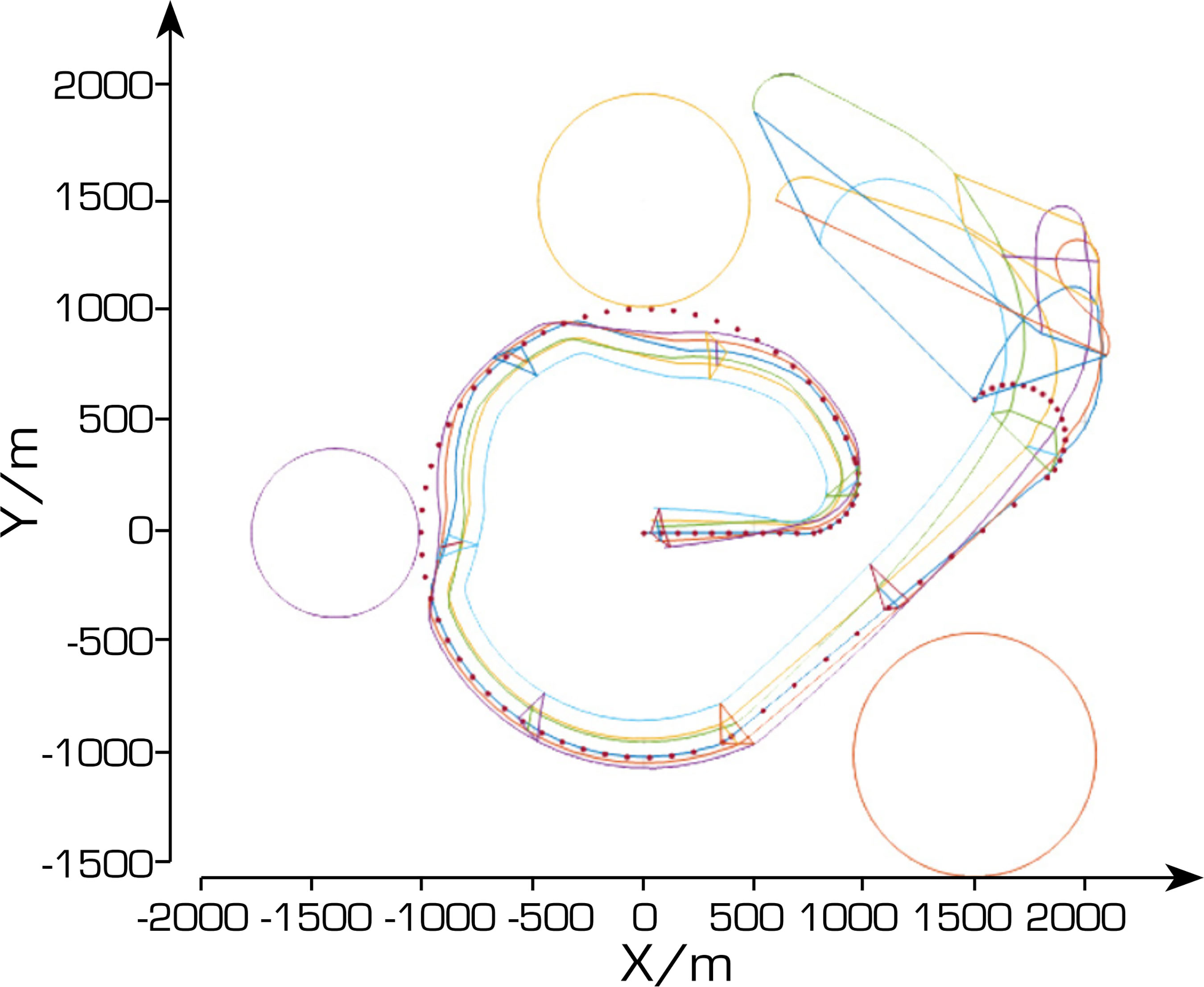
Figures 7 and 8 show the overall flight trajectories and the top view of the three-dimensional simulation environment, respectively. A formation composed of six parafoils is released from an altitude of 2,000 m, with distinct initial positions but sharing the same target area at (0, 0, 0). During the flight, the distance between the parafoil formation and the first mountain remains sufficiently large, and thus no obstacle avoidance maneuver is triggered. When approaching the second and third mountains near the designated target waypoint, the six parafoils exhibit clear avoidance maneuvers. With slight adjustments to the heading, deviating toward the direction away from the mountain can significantly enhance obstacle avoidance performance.

Figure 7
Trajectory diagram of multi-parafoil formations in a three-dimensional environment.

Figure 8
Top view of multi-parafoils formation trajectories.

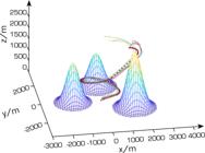
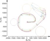
During the return phase, the parafoil formation gradually establishes a triangular formation, maintaining it throughout the subsequent flight while successfully avoiding all three mountain obstacles. Unlike a single parafoil, when the formation approaches a mountain, the inner parafoils (closer to the obstacle) require smaller guidance velocities, whereas the outer parafoils (farther from the obstacle) require larger ones. This adjustment increases the safety distances among parafoils and ensures coordinated obstacle avoidance behavior for the entire formation.

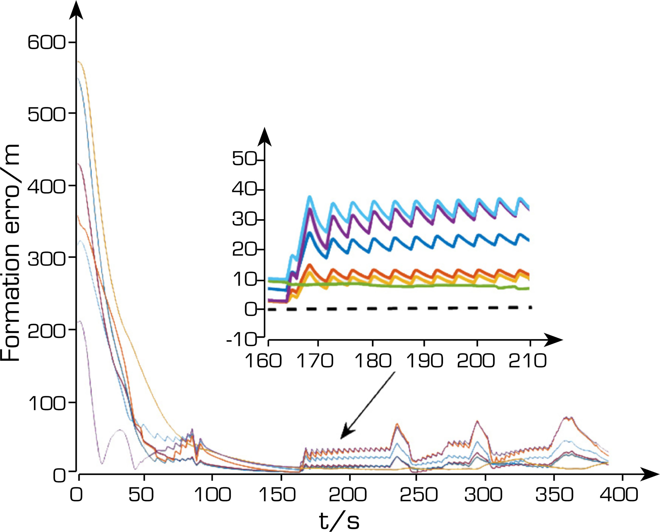
Figure 9 shows the horizontal distance between adjacent parafoils in the formation. Before the parafoils start descending, the horizontal spacing between them is relatively large. During the descent, the inter-parafoil distance gradually decreases, as the six parafoils initially form an irregular configuration that progressively evolves into a stable fixed formation. The minimum inter-parafoil distances remain positive, indicating that no collision occurs and the formation maintains overall stability.

Figure 9
Variation of the distance between adjacent parafoils during flight.

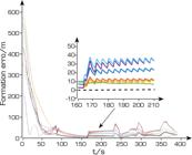
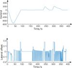
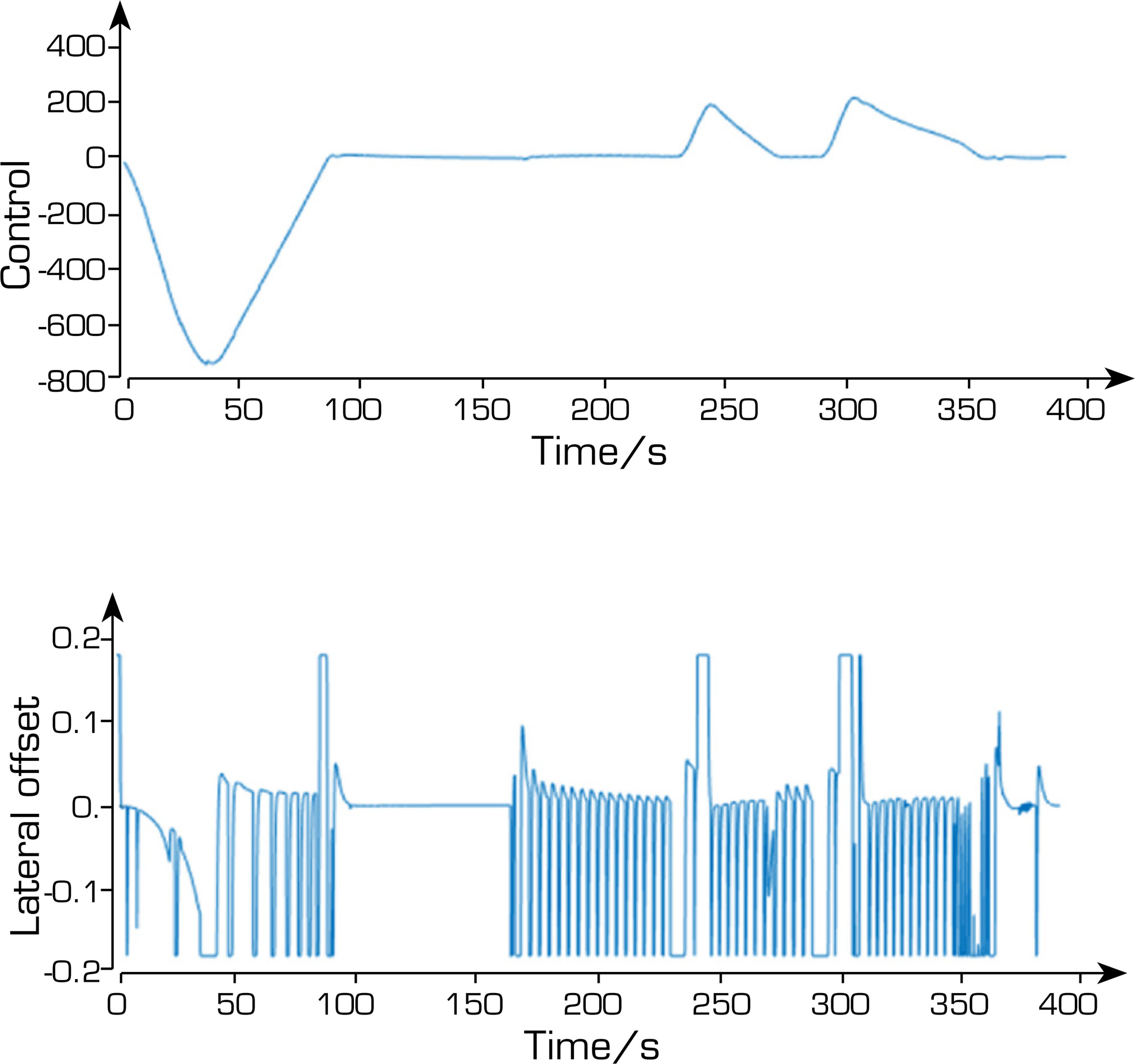
Figure 10 presents the control inputs of the leader parafoil within the formation. It can be observed that at approximately 250 s and 300 s, the control inputs of the leader parafoil experience significant fluctuations. This occurs because the leader parafoil needs to perform obstacle avoidance maneuvers, leading to large variations in its guidance velocity. The lateral deviation exhibits three distinct oscillations: the first arises as the parafoil adjusts its glide angle to initiate descent and maintain formation, whereas the latter two correspond to internal formation adjustments during obstacle avoidance maneuvers. These simulation results demonstrate the effectiveness of the proposed algorithm.

Figure 10
Lateral deviation and control inputs of the leader parafoil.

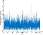
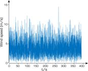
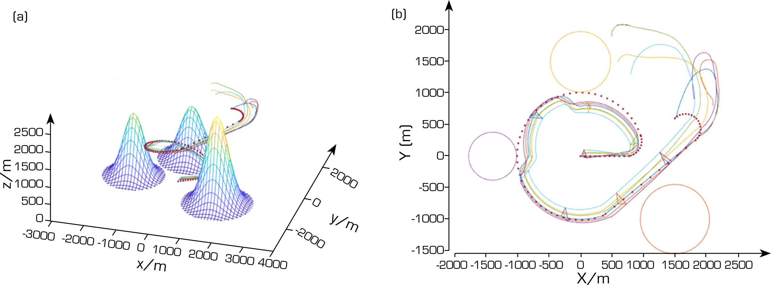
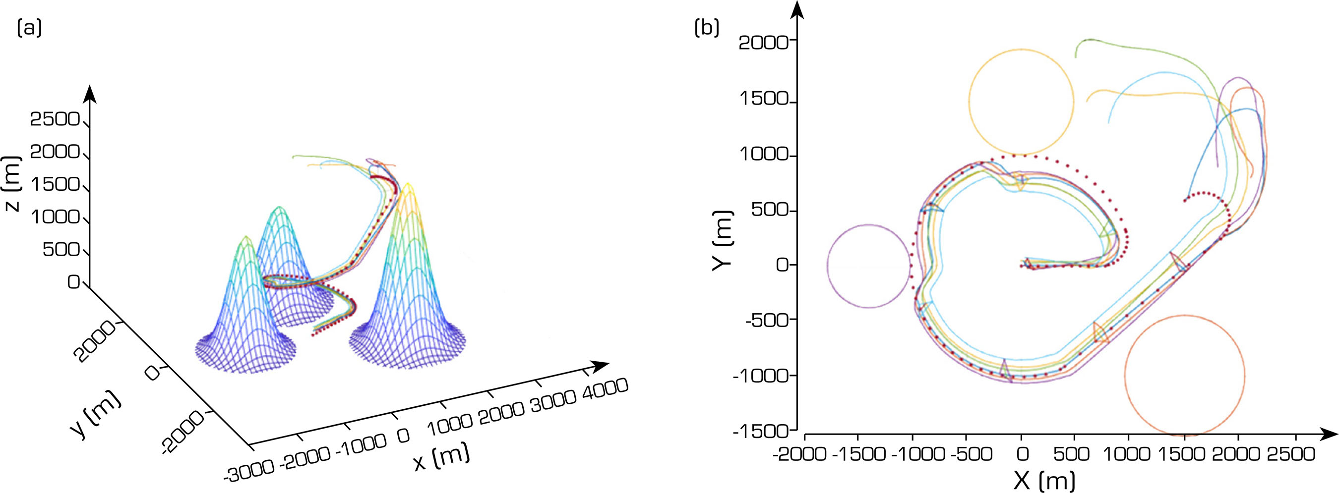
Figures 11a and b and 12a and b show the three-dimensional trajectories and top views of the parafoil formation under mild and strong gust conditions, respectively. To realistically represent the mountainous wind environment, both mild and strong gusts are modeled using randomly generated wind speeds. Under mild gust conditions, the wind speed is primarily concentrated around 2 m·s^-1, whereas under strong gust conditions, it is concentrated around 5 m·s^-1, as illustrated in Figs. 13 and 14. The simulation results demonstrate that the parafoil formation maintains formation consistency under wind disturbances. Although the trajectories of individual parafoils exhibit fluctuations due to wind effects, the overall formation remains coherent, and the relative spacing between parafoils is effectively maintained.

Figure 11
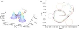
Trajectories of multiple parafoils under mild gust conditions. (a) Three-dimensional trajectories of multiple parafoils under mild gust conditions; (b) Top view of multiple parafoil trajectories under mild gust conditions.

Figure 12
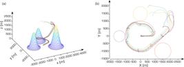
Trajectories of multiple parafoils under strong gust conditions. (a) Three-dimensional trajectories of multi-parafoil formation under strong gust conditions; (b) Top view of multiple parafoil trajectories under strong gust conditions.

Figure 13
Under random mild gust disturbance conditions.

Figure 14
Under random strong gust disturbance conditions.

CONCLUSION

This study investigates trajectory obstacle avoidance in parafoil formations and proposes an innovative spatial velocity model algorithm to address this challenge. Compared with the traditional APF method, the proposed algorithm demonstrates higher computational efficiency and greater flexibility, effectively alleviating the local minimum issue inherent in conventional approaches. By integrating consensus-based formation control theory and adopting a leader-follower strategy, the method enables the parafoil formation to maintain its configuration during obstacle avoidance and to remain within the designated operational range. Under wind disturbances, although minor fluctuations appear in individual parafoil trajectories, the overall formation maintains stable and safe separation distances. Simulation results indicate that, when the formation maintains a sufficient distance from obstacles, the parafoils preserve their flight path without avoidance actions. As the formation approaches obstacles, the system successfully avoids obstacles while maintaining formation integrity.

ACKNOWLEDGEMENTS

Not applicable.

• FUNDING
  Not applicable.
• DECLARATION OF USE OF ARTIFICIAL INTELLIGENCE TOOLS
  Artificial intelligence tools were used only to assist with language polishing and translation during the preparation of this manuscript. All scientific content, including the research design, data analysis, results, and conclusions, was created entirely by the authors.
• Peer Review History
  Single Blind Peer Review.

DATA AVAILABILITY STATEMENT

All data sets were generated or analyzed in the current study.

REFERENCES

• Chen Q, Zhao M, Jin Y, Yao M (2019) Multi-objective cooperative paths planning for multiple parafoils system using a genetic algorithm. J Aerosp Technol Manag 11: e0419. https://doi.org/10.5028/jatm.v11.1005
  » https://doi.org/10.5028/jatm.v11.1005
• Gao H, Tao J (2022) A novel trajectory planning method for parafoil airdrop system based on geometric segmentation strategy. Math Comput Appl 27(5):75. https://doi.org/10.3390/mca27050075
  » https://doi.org/10.3390/mca27050075
• Huang H, Ma WH, Li JC, Fang Y (2024) Intelligent obstacle avoidance control of UAV formation in unknown environments. J Tsinghua Univ (Sci Technol) 64(2):358-369.
• Jia YN, Jiao, Chen X, Zhang XX (2024) Countermeasure strategies of multi-UAV swarm based on dynamic Bayesian networks. J Eng Sci 46(7):1216-1226. https://doi.org/10.13374/j.issn2095-9389.2023.10.12.001
  » https://doi.org/10.13374/j.issn2095-9389.2023.10.12.001
• Li J, Zi SK, Lu XT (2024a) Improved artificial potential field method for UAV swarm combat strategy. Radio Eng 54(8):1970-1977. https://www.cjwk.cn/journal/guidelinesDetails/1818855655143030784
  » https://www.cjwk.cn/journal/guidelinesDetails/1818855655143030784
• Li YH, Zhao M, Chen Q, Wang ZL (2021) Combined trajectory planning of parafoil systems in complex environments. Acta Aeronaut Astronaut Sin 42(6):545-556. https://doi.org/10.7527/S1000-6893.2020.24566
  » https://doi.org/10.7527/S1000-6893.2020.24566
• Li ZH, Nan Y, Wan JC (2024b) Trajectory planning of parafoil system based on the original natural algorithm. Ship Electron Eng 44(3):31-36. https://c.wanfangdata.com.cn/magazine/jcdzgc/?isSync=0&issueNum=03&page=1&publishYear=2024&tabId=article
  » https://c.wanfangdata.com.cn/magazine/jcdzgc/?isSync=0&issueNum=03&page=1&publishYear=2024&tabId=article
• Lu WT, Sun H, Teng HS (2022) Research on intelligent cooperative control of multi-parafoil system. Spacecraft Recovery Remote Sens 43(5):36-47. https://doi.org/10.3969/j.issn.1009-8518.2022.05.004
  » https://doi.org/10.3969/j.issn.1009-8518.2022.05.004
• Lu XD, Wang YM, Wang W (2024) Task assignment algorithm for UAV cooperative interception under communication constraints. Aviat Sci Technol 35(4):18-24. https://doi.org/10.19452/j.issn1007-5453.2024.04.003
  » https://doi.org/10.19452/j.issn1007-5453.2024.04.003
• Ma W, Ding F, Zhao ZY, Liu Q (2024) Mission planning strategy of UAV swarm based on user clustering. Radio Commun Technol 50(3):528-534. https://xueshu.baidu.com/usercenter/paper/show?paperid=1x440a60d1620ct0aw160tm007322562
  » https://xueshu.baidu.com/usercenter/paper/show?paperid=1x440a60d1620ct0aw160tm007322562
• Qin WJ, Lin Y, Qi GQ (2018) Consensus-based UAV formation and collision avoidance. Electron Des Eng 26(9):83-85. https://xueshu.baidu.com/usercenter/paper/show?paperid=227b5e5a4051b3279733dcb79cced6e3
  » https://xueshu.baidu.com/usercenter/paper/show?paperid=227b5e5a4051b3279733dcb79cced6e3
• Ren PB (2023) Research on cluster obstacle avoidance algorithm based on artificial potential field. Mod Navig 14(1):65-69. https://www.cqvip.com/journal/70785X/
  » https://www.cqvip.com/journal/70785X/
• Sun Q, Yu L, Zheng Y, Tao J, Sun H, Sun M, Dehmer M, Chen Z (2022) Trajectory tracking control of powered parafoil system based on sliding mode control in a complex environment. Aerosp Sci Technol 122:107406. https://doi.org/10.1016/j.ast.2022.107406
  » https://doi.org/10.1016/j.ast.2022.107406
• Sun QL, Yang JS, Sun H (2024) Key technologies for autonomous recovery of parafoil systems: A review. J Natl Univ Def Technol 46(4):1-15. https://doi.org/10.11887/j.cn.202404001
  » https://doi.org/10.11887/j.cn.202404001
• Wang Y, Yang CX (2024) Study on aerodynamic characteristics of parafoil canopy based on LBM. Sci Technol Innov Appl 14(6):1-6. https://www.knowcat.cn/p/20240524/1194976.html
  » https://www.knowcat.cn/p/20240524/1194976.html
• Zhang YC, Duan HB, Wei C (2024) Digital-twin-based formation obstacle avoidance of UAV swarm using deep reinforcement learning. J Eng Sci 46(7):1187-1196. https://doi.org/10.13374/j.issn2095-9389.2023.09.28.005
  » https://doi.org/10.13374/j.issn2095-9389.2023.09.28.005
• Zhao J, Zhang X, Chi P (2024) Self-adaptive formation control and dynamic path planning for air-ground heterogeneous swarm. Acta Aeronautica et Astronautica Sinica 45(16):207–226. https://doi.org/10.7527/S1000-6893.2024.29809
  » https://doi.org/10.7527/S1000-6893.2024.29809
• Zhao L, Tao J, Sun H, Sun QL (2023) Dynamic modeling of parafoil system based on aerodynamic coefficients identification. Automatika 64(2):291-303. https://doi.org/10.1080/00051144.2022.2145697
  » https://doi.org/10.1080/00051144.2022.2145697
• Zhao LG, He WL, Du YJ (2022) Dynamic parameter identification of parafoil system based on sensitivity analysis. Spacecraft Recover Remote Sens 43(1):26-39. https://doi.org/10.3969/j.issn.1009-8518.2022.01.003
  » https://doi.org/10.3969/j.issn.1009-8518.2022.01.003
• Zheng Y, Tao J, Sun Q, Sun H, Chen Z, Sun M (2023) Deep-reinforcement-learning-based active disturbance rejection control for lateral path following of parafoil system. Sustainability 15(1):435. https://doi.org/10.3390/su15010435
  » https://doi.org/10.3390/su15010435
• Zhou YY, Zhao M, Wang C (2024) Three-dimensional trajectory tracking control of parafoil system based on bilinear ADRC. Mach Manuf Autom 53(1):255-259. https://www.jxzzyzdh.com/Uploads/Download/2024-02-26/65dc2a010e886.pdf
  » https://www.jxzzyzdh.com/Uploads/Download/2024-02-26/65dc2a010e886.pdf

Edited by

• Section editor:
  Luiz Martins-Filho https://orcid.org/0000-0002-7287-5979

Publication Dates

• Publication in this collection
  20 July 2026
• Date of issue
  2026

History

• Received
  30 Oct 2025
• Accepted
  15 Apr 2026