Analysis of Emission Files Generated by a Global Model for Air Quality Simulation in the State of Rio de Janeiro

Abstract

Emission inventories are essential tools for air quality management. However, the state of Rio de Janeiro lacks a comprehensive inventory. Consequently, global models such as EDGAR (Emission Database for Global Atmospheric Research) become an attractive alternative. This study aims to analyze data on nitrogen oxides (NOx) and volatile organic compounds (VOCs) and compare them with existing data. To achieve this, a 3 × 3 km simulation grid centered on the state of Rio de Janeiro was constructed. Meteorological fields were generated using the Weather Research and Forecasting model, while emission data were obtained from EDGAR. The simulation period spanned 34 days in 2018. Emissions were analyzed for NOx and VOCs, and compared to mobile source inventory data from the State Environmental Institute of Rio de Janeiro. Sectoral contributions to NOx emissions revealed that industry, navigation, and energy were the dominant sources. For VOCs, the primary contributors were industry, residential sources, and transportation. The comparison with State Institute for the Environment of Rio de Janeiro (INEA-RJ) data indicated that the model underestimated NOx and VOC emissions by approximately 38 and 48%, respectively. Despite the underestimation, the model effectively captured the regional emission characteristics, highlighting its potential as a tool for emission analysis without a comprehensive local inventory.

Keywords:
emission inventory; EDGAR; SMOKE; chemical speciation; Rio de Janeiro

Introduction

Emission inventories are essential tools for air quality management.¹ They provide critical data on various economic activity sectors and their associated pollutant emissions, enabling a comprehensive diagnosis of pollutants influencing the atmospheric dynamics of the region and their potential impacts on air quality.² Moreover, these inventories facilitate early warnings about critical pollution episodes and help identify the main sources contributing to poor air quality.³ Such assessments must encompass all locations affected by emissions, ranging from continental and national scales to state and local levels. Many countries maintain both regional and national emission inventories. Kawashima et al.⁴ analyzed the main industrial sources in Brazil, primarily assessing the importance of the industrial sector in the Southeast region. Loriato et al.⁵ also using the Sparse Matrix Operator Kernel Emissions (SMOKE) model, developed emission data from the Vitória’s Metropolitan Area inventory to analyze the contributions of emissions to the local atmosphere.⁵-⁹

Brazil has emission inventories for some metropolitan regions but still lacks a unified national inventory covering all or the most significant emission sectors in the country. Furthermore, the existing inventories lack standardization in aspects such as the types of sources evaluated, pollutant criteria, frequency of updates, estimation methods, and the application of emission factors.⁵,⁶ Additionally, few studies comprehensively and detailed address entire states.¹⁰,¹¹

The state of Rio de Janeiro, one of Brazil’s largest economies and part of the country’s main economic axis hosts a vast and diverse industrial base alongside a high population density, resulting in a significant number of mobile emission sources. Mapping these sources is thus essential for understanding air quality in the region.⁶,¹²,¹³ However, Rio de Janeiro lacks comprehensive emission source inventories across various sectors. The most recent inventory, conducted in 2024, accounted solely for mobile sources and covered only the metropolitan region. Consequently, there is a notable lack of data not only for the transportation sector but also for other emission sectors.¹⁴

As mentioned, understanding local air pollution relies heavily on national, regional, or local emission inventories. However, in the absence of comprehensive data, global models become a viable alternative. For instance, EDGAR (Emission Database for Global Atmospheric Research) is a global emissions model that integrates emission estimates and available national inventories, compiling these into a global dataset with sector-specific information. For countries like Brazil, which do not produce national inventories, EDGAR employs a numerical approach.⁷,¹⁵,¹⁶ This method leverages activity data, applying mathematical formulas that incorporate local emission factors, country-specific activity characteristics, pollutant abatement mechanisms, and end-of-process technologies. Crippa et al.¹⁶ provides a detailed explanation of these methodologies in their study.

EDGAR data is adjusted to produce values compatible with Chemical Transport Models (CTMs) using SMOKE, an emissions processor that adapts the data through matrices divided into three stages: temporal profile, spatial profile, and chemical speciation. Among these, chemical speciation is a critical step as it defines the chemical species that will participate in local reactions.¹⁷ These profiles are developed for pollutants comprising various species within their class, such as particulate matter and organic compounds. Based on the activity type, a set of compounds is allocated, representing the chemical profile for the specific emissions category.¹³

Volatile organic compounds (VOCs) exhibit a wide variety of sources, chemical structures, reactivity, and toxicity. Understanding these compounds is therefore crucial for studying the chemistry of the local atmosphere.¹⁸ Geraldino et al.¹⁹ highlighted that Rio de Janeiro is characterized by significant VOC emissions, with these pollutants exerting a direct and proportional influence on ozone formation in the city. This underscores the importance of studying these compounds in the region. Consequently, developing an inventory and understanding the organic compounds specific to the state of Rio de Janeiro is essential for comprehending the atmospheric chemistry of the study area.⁴,²⁰,²¹

Therefore, the objective of the present study is to evaluate the performance of the global EDGAR model in generating emission data for ozone precursor pollutants, with a particular focus on volatile organic compounds, for the Rio de Janeiro region.

Experimental

The methodology of this study consists of two main stages. The first stage involves characterizing the emissions from the global model and comparing them with the emissions available for the state of Rio de Janeiro in the mobile source inventory provided by the State Institute for the Environment of Rio de Janeiro (INEA-RJ).¹³ The project employed a remote computer to perform simulation controls located at the State University of Rio de Janeiro (UERJ), Resende campus, communicating with the cluster hosted at the Federal University of Minas Gerais (UFMG), Pampulha campus, in Belo Horizonte, provided by the GPAMA research group (Air Pollution and Applied Meteorology Research Group).

The second stage evaluates the influence of the chemical profiles applied to the modeled emissions, focusing on the concentration of each VOC species. Figure 1 provides a schematic diagram of the methodology of the study.

Figure 1
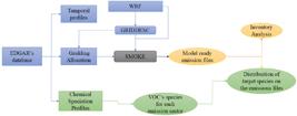
Schematic diagram of the data analysis structure according to the two segments of the study.

The emission processing requires four main models/processors. First, EDGAR, as the global model, generates emission data for the primary pollutants. Second, WRF (Weather Research and Forecasting) is responsible for generating meteorological data and the simulated domain. The third model is MCIP (Meteorological-Chemical Interface Processor), a processor for the CMAQ (Community MultiScale Air Quality Model) photochemical model, which converts meteorological fields into formats compatible with the emission processor and generates the grid data file, called GRIDDESC. This file is responsible for the spatial allocation of the emissions. Finally, SMOKE, the emissions processor, combines the EDGAR data with the meteorological fields and spatial data to allocate emissions to sources and chemically speciate the species.¹⁷

The domain covers the state of Rio de Janeiro at its center and was simulated for 34 days (August 29-October 1, 2018). The results of the WRF validation according to ENVIRON²² and AMMM²³ can be found in the Supplementary Information (SI) section.

For text editing, AI was used in: grammar correction, coherence, cohesion, and English language translation.

Emissions inventory

EDGAR generates values for the primary pollutants by activity. These values were extracted for the following pollutants: SO₂, NOx, CO, CH₄, PM₁₀, PM_2.5 (particulate matter), NH₃, EC (elemental carbon), OC (organic carbon), and NMVOC (non-methane volatile organic compounds). The sectors chosen for the study were: industry, energy, solid waste, residences, transport, other transport sectors, international aviation, and international shipping. The selection of these eight sectors was mainly based on the characterization of the study area. The state of Rio de Janeiro has a strong industrial profile, focused on the oil and gas industry, with the presence of thermoelectric plants in some regions and port areas, such as the metropolitan region of Rio de Janeiro and the Angra dos Reis region. Additionally, the state has petroleum distribution terminals throughout its extension and presents a relatively low agrarian profile, consisting mainly of small farmers who generate lower emissions from this sector. The relevance of emissions from sectors like energy and transport is much greater in mass compared to evaporative emissions, for example. More specific sectors such as solvents and livestock were not included in the scope of the study, mainly due to the lack of detailed emissions data from EDGAR, which would likely result in less significant contributions to the modeled emissions or lead to errors. Furthermore, due to processing speed, the simulation time and computational space needed also played a role in limiting the inclusion of additional sectors, as each sector for a month of simulation generates files that take days to simulate, with sizes on the order of tens of gigabytes.¹⁶

The results obtained from the simulation were extracted for the area of the state of Rio de Janeiro and surrounding regions. Figure 2 shows the modeled grid.

Figure 2
Simulation domain with a 3 km × 3 km resolution generated by the WRF4GIS module in the QGIS 3.40.3 software.

The data for each pollutant were obtained from the model’s website.²⁴Table 1 shows the simulation data. The emission data processing was done for the tropospheric ozone simulation in the state of Rio de Janeiro; therefore, the validation and emission study focus only on the precursor pollutants responsible for its generation and accumulation.

Table 1
Model configurations for the generation of emission files

Simulation configuration
Horizontal grid resolution / km	3 × 3
Vertical grid resolution / layer	40
Temporal allocation	August 29-October 1, 2018
Chemical mechanism	Carbon Bond 2006
Emission processor	Sparse Matrix Operator Kernel Emissions (SMOKE)

After downloading the emission data from the database, they were processed by SMOKE (Sparse Matrix of Operator Kernel Emissions) with the aim of spatially and temporally allocating the emissions according to the chemical profiles. These steps are presented in the sequence.

Spatial allocation

The spatial allocation of the data is based on the grid obtained through the QGIS extension, GIS4WRF. These grid data are then processed with MCIP, which generates a GRIDDESC file. This file presents the grid size and its values in coordinates, as well as row and column numbers. Thus, SMOKE can generate the data according to the location based on the matrix scheme. Table 2 shows the configuration of the studied domain.

Table 2
Spatial data of the grid and matrix configuration utilizing in Sparse Matrix Operator Kernel Emission Model (SMOKE)

Parameter
Conformation	Lambert
True latitude 1	-19.800
True latitude 2	-26.750
Longitude	-43.200
Number of rows	138
Number of columns	150

The vertical levels were constructed according to profiles for industry, navigation, aviation, and energy. For the navigation and aviation profiles, the allocation generated by the EDGAR_HTAP (Emissions Database for Global Atmospheric Research with Hemispheric Transport of Air Pollution) was used. For industry and energy, the chimney heights presented in the Environmental Impact Assessments (EIAs) of some industries in the Baixada Fluminense region were used as the basis for the vertical layers. Table 3 shows how many layers each profile was divided into, along with the maximum and minimum heights of each.

Table 3
Vertical profile of sectors with vertical stratification, showing the number of layers, maximum and minimum height for each sector

Profile	Number of layers	Minimum high	Maximum high
Industry	5	0	200
Energy	5	0	200
Shipping	8	0	470
Aviation	10	0	2500

Temporal allocation

For the temporal allocation, weekly, daily, and monthly profiles were used. These profiles account for the behavior of the pollutant, whether it is daily or seasonal. For example, NOx emissions are higher in the energy sector during the summer months, when there is greater consumption of cooling devices and electric showers in tropical countries such as Brazil.

For each sector, profiles available on the EDGAR platform were gathered.²⁴

Each sector has a unique monthly profile and a unique weekly profile according to its characteristics. However, daily profiles vary depending on certain sectors.

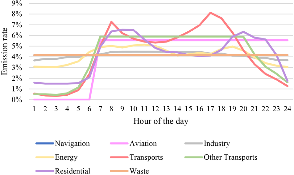
The sectors of industry, energy, aviation, solid waste, navigation, and other transport are consistent throughout the weekdays. However, the transport and residential sectors exhibit variations, with specific profiles applied for weekdays and weekends. Pollutants with specific hourly emission profiles for weekdays need to be distinguished from others, as their emission rates vary between weekdays and weekends. This distinction is due to pollutants such as NOx, which show a shift in their peak hours, as car users tend to leave at later times compared to their workday schedules. The same applies to the residential sector, where during weekends, the population spends more time at home, resulting in increased use of appliances such as stoves. The daily temporal profiles for the transport and residential sectors are available in the SI section.

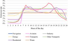
For the precursors, the diurnal emission cycles followed the characteristic patterns of each sector for both precursors. The selection of daily emission profiles was made by the author based on the data presented in Table 4 and the values available on the EDGAR HTAP website, version 3. Figure 3 shows the emission profiles for each sector considered in the simulation.³,¹⁶

Table 4
Description of the chemical profiles used for the VOC speciation for each modeled sector

Chemical profile	Description
Industry	generic profile for any volatile organic compounds (VOC) emitting from industry sector obtained from the SPECIATE repository of the United States of America Environment Protection Agency (US-EPA); based on the steel, coke processing and petrochemical sectors obtained on Hemispheric Transport Atmospheric Pollution Research (HTAP) version 3 profiles16
Energy	profile based on thermoelectric power plants for energy generation; allocation performed according to the national balance of 202126 the fuels used are: 43% petroleum, 32% sugarcane bagasse, 7% coal, and 1% residual oil
Navigation	profile based on the US-EPA SPECIATE repository for commercial ships in international shipping, but with specific allocation of 85% of emissions derived from the main engine and 25% from the auxiliary engine, following the study by Sui et al.;27 the profile primarily reflects diesel engines, with VOC and NOx emission rates corresponding to this type of fuel
Aviation	profile obtained from the US-EPA SPECIATE repository for takeoff and landing of large international flights
Residential	profile obtained for households using gas stoves; the allocation was constructed based on the use of liquefied petroleum gas in households in Mexico City, according to Luis et al.28 VOC emissions were estimated based on the chemical composition of the gas, while NOx emissions were derived from stove combustion
Waste	the organic compounds were speciated based on emissions from landfills and sewage treatment. The emission fractions were divided 50% for sewage treatment and 50% for landfill emissions for VOCs, excluding methane
Transports	profile based on the vehicular emission study by Dominutti et al.29 considering light and heavy-duty vehicles operating in the São Paulo metropolitan area
Other transports	obtained from HTAP version 3 data, the emission profile for gas pipelines and oil pipelines16 with a primary focus on VOC evaporation during transport

Figure 3
Emission rate of the simulated pollutants by hour of the day.

Chemical speciation

For the chemical speciation, the profiles obtained were sourced from the SPECIATE platform of the United States of America Environmental Protection Agency (EPA).²⁵ For certain sectors, the speciation was adjusted in a specific manner to better align with the Brazilian reality. For other sectors, the chemical profiles were obtained from academic studies designed to specify pollutants with local characteristics.

The chemical profiles obtained from SPECIATE are included in the SMOKE database, allowing the processor to correlate them with the species in the inventory using their respective codes and apply the allocation factors. Allocation factors are created by the user based on local factors or scientific studies. Typically, speciation is applied only to volatile organic compounds (VOCs) and particulate matter with an aerodynamic diameter smaller than 2.5 µm, due to the complexity of these pollutants, as chemical transport models can only process species. The division is applied in a way that replicates the behavior of the pollutant mixture when emitted. For example, VOCs present in liquefied petroleum gas (LPG) have distinct compositions in each country. In Brazil, the mixture consists of butane and propane, with a higher proportion of propane. Therefore, the VOCs in the residential sector, which uses this type of gas, should have higher percentages of butane and propane compared to other organic compounds.

For the remaining pollutants, the conventional profile is applied, where the pollutant maintains its original structure, meaning 100% of its allocation corresponds to the form presented. For example, nitrogen monoxide will remain 100% nitrogen monoxide, as the reactions in which it participates involve it in the same form.

Since the inventory was built for a simulation of tropospheric ozone concentrations, only the allocation of organic compounds was considered. Table 4 presents the chemical profiles of each sector and the description of the allocation method.

Emission validation

Due to the lack of updated emission inventories made available by environmental agencies at both federal and state levels, the validation of the emission processor is limited, particularly because of the scarcity of sector-specific data and the unavailability of time series with monthly or weekly resolution, such as those provided by the EDGAR inventory. Given this context, emission validation was carried out based on the mobile source inventory developed by the State Environmental Institute (INEA) for the year 2013,¹³ as it is temporally closer to the study period. Although a more recent version of the inventory exists for the base year 2023, the 2013 version was chosen to ensure greater compatibility with the analyzed year.

In the absence of normative criteria or specific reference values for emission validation, commonly used statistical metrics in air quality model performance evaluation were adopted, including the normalized mean bias (NMB), the normalized mean error (NME), and the root mean square error (RMSE).²²,³⁰

The INEA inventory provides annual emission data (in tons per year), disaggregated by road type and covering the Metropolitan Region of Rio de Janeiro. For comparison purposes, the data were aggregated to obtain the total annual emissions corresponding to the model domain. The simulation data, in turn, were initially generated for the study month and subsequently extrapolated to annual estimates, thus allowing a direct comparison between the two datasets.

Comparison scenarios

To improve the visualization of inventory data and enable interpretation based on real-world information, comparisons were made using three hypothetical scenarios between the transport sector emissions from the EDGAR inventory and the emissions inventory of the Metropolitan Region of Rio de Janeiro for the base year 2013. Due to the lack of data from other sources, the state of Rio de Janeiro, through its State Environmental Institute (INEA-RJ), has only developed an inventory for mobile sources, which was recently updated for the base year 2022. However, the 2013 inventory was selected for this evaluation due to its greater temporal proximity to the extrapolated data.¹³

For comparison purposes, the 2013 mobile source emissions were linearly extrapolated based on the increase in the light vehicle fleet over time, without accounting for changes in fuel types, fleet aging, or the introduction of cleaner technologies in newer vehicles. An overall increase of 22.23% in the fleet from 2013 to 2018 was identified. This percentage was calculated based on the growth of the vehicle fleet in the city of Rio de Janeiro during this five-year period, considering the total number of vehicles-a figure close to that reported by the National Confederation of Municipalities.³¹ This percentage increase was then applied to the total emissions of the pollutants.

In addition, since the modeled emissions correspond to the simulation period, they were also extrapolated to represent annual emissions by multiplying the results by 12 (months), enabling a more direct comparison. To mitigate potential errors from the linear fleet projection, three distinct growth scenarios were developed: one assuming the fleet increase in the state mirrors that of the city of Rio de Janeiro; a second, more conservative scenario that assumes a smaller increase in emissions due to technological advancements and fleet age shifts; and a third, more pessimistic scenario assuming higher emissions proportional to the fleet growth.

Results and Discussion

Chemical profiles

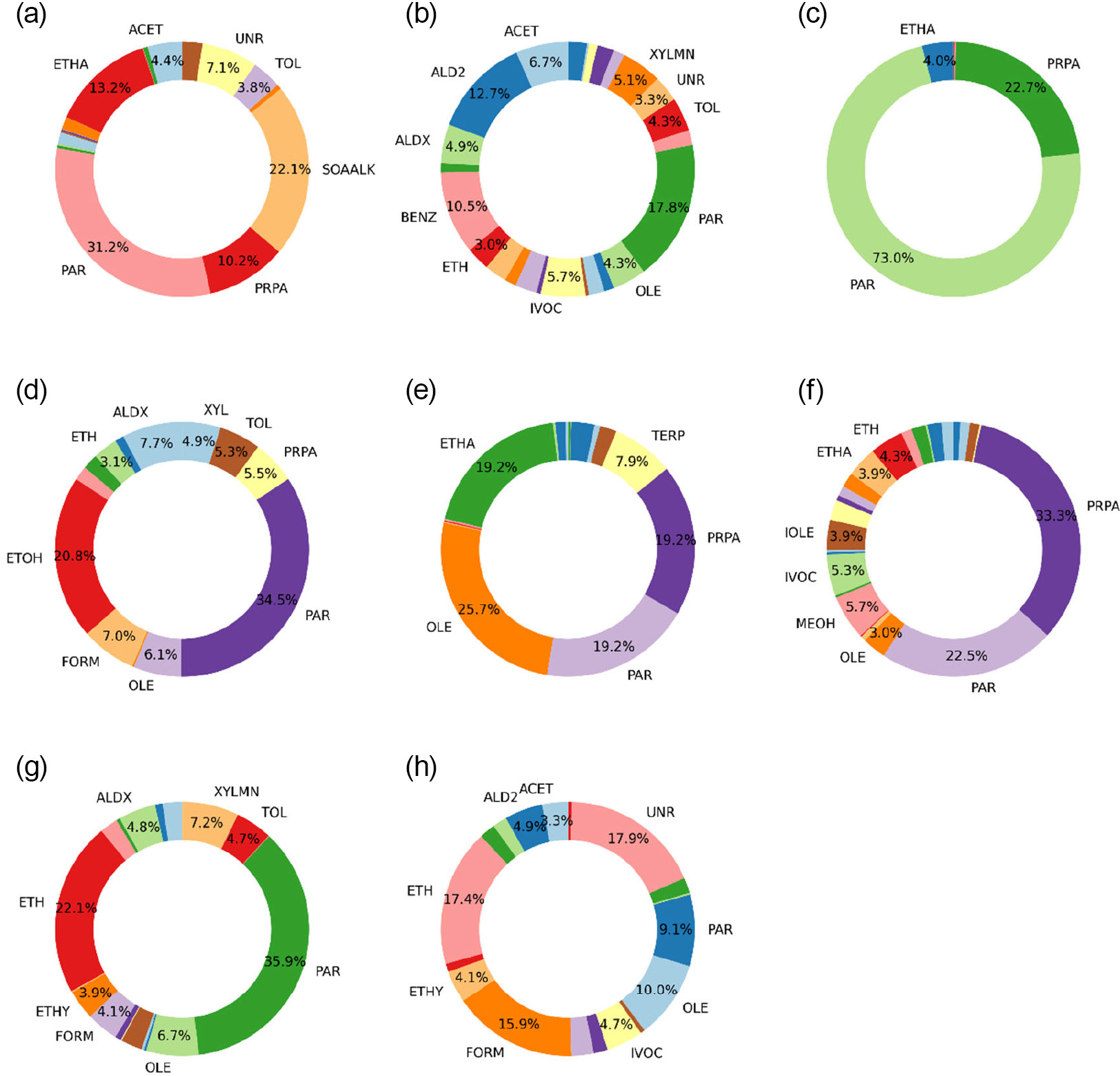
Figure 4 shows the percentage distribution of the main species considered in the chemical profiles for the different emission categories of the inventory.

Figure 4
Percentage of the main organic species within the respective chemical profile for each sector. (a) Industry, (b) energy, (c) other transport, (d) road transport, (e) waste, (f) residential, (g) international shipping, (h) international aviation. Organic compounds: ACET: acetone; ALD2: aldehydes; ALDX: higher aldehydes; ETHA: ethane; ETH: ethene; ETHY: ethyne; ETOH: ethanol; FORM: formaldehyde; IVOC: semi-volatile organic compounds; MeOH: methanol; IOLE: intermediate olefines; OLE: olefines; PAR: paraffins; PRPA: propane; SOAALK: secondary aerosol’s alkene products; TOL: toluene; TERP- terpenes; UNR: unreactive; XYLMN: xylenes.

Paraffins (PAR) are the most prevalent species in all chemical profiles, which is consistent with reality, as most sectors burn fossil fuels derived from petroleum and/or emit organic vapors during their processes, such as sanitary landfills, sewage treatment plants, and pipelines. Geraldino et al.¹⁹ showed that in their simulation, the presence of alkanes in the VOC mass in Rio de Janeiro was also the highest. Using the Statewide Air Pollution Research Center Chemical Mechanism version 99 (SAPRC-99), the researchers also presented their speciation, considering the predominance of these species.¹⁹

There is a wide diversity of species in the emission files, which is expected due to the variety of organic compounds resulting from the processes. The transport sector, due to its significant impact on emissions in the state of Rio de Janeiro, becomes relevant, showing a high percentage of emissions from paraffins (PAR), ethanol (ETOH), formaldehyde (FORM), and olefins (OLE). Formaldehyde, paraffins, and olefins have a significant potential for ozone formation, which makes mobile sources the largest contributors to the pollutant in the region. Carvalho et al.³² also confirms the presence of xylenes (XYLMN) and toluenes (TOL), as these are found in their study in locations within the city of Rio de Janeiro.³²

The “other transport” sector, such as gas and oil pipelines, shows a coherent speciation, as these transportation methods primarily use petroleum derivatives, particularly automotive fuels and LPG. Therefore, PAR, propane, and ethane are their main emissions. Similarly, the residential sector in Brazil is largely characterized by the use of LPG for cooking and, in some regions, for heating shower and sink systems, which results in emissions of propane (PRPA) and paraffins (PAR). McDuffie et al.,³³ using EDGAR for the African continent, confirm that the residential sector is one of the largest contributors of VOCs, primarily due to the fuels used in households.³³

Other relevant species that appear in some profiles are aldehydes (aldehydes (ALD2), higher aldehydes (ALDX), formaldehyde (FORM)). These species are not present in the solid waste, other transport, and residential profiles. In the first case, it is mainly because incinerators were not considered, only anaerobic respiration processes, which result in lower percentages of these compounds. In the latter two sectors, it is because they are primarily focused on emissions of hydrocarbons derived from petroleum. However, when considering the other sectors, these species always correspond to more than 5% of the emissions in the profiles.

Rowlinson et al.³⁴ showed that the presence of ethane and propane in the speciation profiles plays an important role in the lifetimes of organic species in the troposphere, influencing intermediate species and ozone accumulation. Therefore, it is important to seek a more specific chemical speciation for the location, as this brings the model performance closer to the observed data. da Costa et al.³⁵ confirm this in their systematic review, where the presence of local inventories with more specific chemical profiles leads to more reliable results in chemical transport models.

Thus, two criteria were established for the analysis of species. The first, based on the species with the highest percentage of occurrence in the profiles, and the second, gathering the species with significant reactivity in the troposphere. These are: paraffins (PAR), olefins (OLE), propane (PRPA), ethene (ETH), formaldehyde (FORM), acetone (ACET), and acetaldehyde (ALD2).

Emissions by sectors

Figures 5 and 6 show the concentrations for a single day, generated by SMOKE for the different sectors and for the two pollutants of interest. The figures were created to visualize the spatial allocation of emissions for each sector.

Figure 5
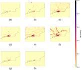
Spatial allocation of NO emissions (mol s^-1) in time step 0 distributed spatially within the simulation domain for each sector. (a) Energy, (b) industry, (c) residential, (d) waste, (e) transport, (f) other transport, (g) international aviation, (h) international shipping.

Figure 6
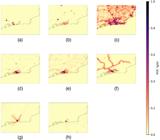
Spatial allocation of VOC emissions (g s^-1) in time step 0 distributed spatially within the simulation domain for each sector. (a) Energy, (b) industry, (c) residential, (d) waste, (e) transport, (f) other transport, (g) international aviation, (h) international shipping.

Even in mol s^-1, the distribution of NO emissions according to each sector can be observed, with the highest emissions concentrated in the center, represented by the metropolitan region of Rio de Janeiro. For NO, the industrial and energy sectors are point sources, only observable as spots on the map. On the other hand, the transportation sector, due to combustion processes, shows greater detail along the roads. The aviation sector, limited to takeoff and landing, exhibits a diffusion of emissions in a diagonal pattern, following the flight trajectories.

Regarding the VOCs, the residential sector stands out, primarily due to the explanation provided earlier. The speciation of LPG highlights the emissions from residences, especially for organic compounds. The “other transport” sector, also shows significant emissions.

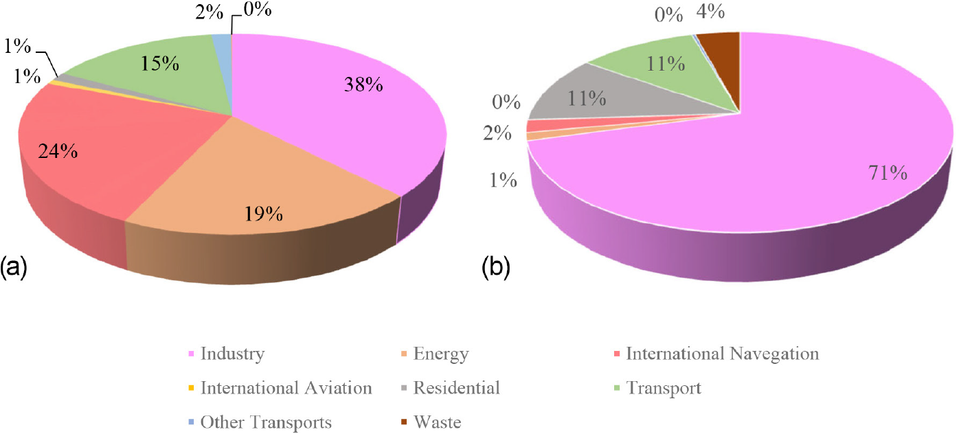
Figure 7 presents the contribution profiles for the main pollutants according to each sector. The percentages take into account the total gross emissions of each pollutant throughout the simulation period.

Figure 7
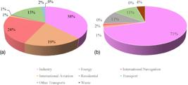
Contribution of pollutant modeled emissions by sector. (a) Emissions of NOx; (b) emissions of COV.

Regarding the contribution percentage, it can be observed that NOx emissions are dominated by the industry, energy, and shipping sectors. These sectors have high and constant emissions according to the established profiles. Rio de Janeiro, being a southeastern state with a large number of industries and port terminals, particularly in the metropolitan region and northern Fluminense, leads to increased emissions from both the shipping and industrial sectors. Another important factor is the presence of thermoelectric plants in areas around the state and in neighboring regions. McDuffie et al.³³ found similar contribution percentages in Africa and India, with the exception of the transportation sector in Africa. The higher presence of diesel-powered vehicles in Africa leads to higher NOx emissions compared to the industrial sector. This resulted in a larger contribution from the transportation sector compared to the industrial sector in their study. Since Africa provides more detailed data on the fuels used in fleets, it is likely that the transportation sector in the present study generates a lower value.³³ This results in the transportation sector appearing in a lower position compared to industry and energy, despite the significant vehicle fleet in the state of Rio de Janeiro. Puliafito et al.¹⁵ also confirmed the greater influence of the transportation sector in EDGAR, which results in a higher contribution to NOx emissions in Argentina. However, in their study, the energy sector is the largest contributor to NOx emissions.¹⁵

According to Alamos et al.,⁸ the largest emissions come from the transportation sector in Chile, followed by the energy and industrial sectors. This is likely due to the greater level of detail in sector-specific data. In their study, a more distinct differentiation was observed in the contributions using local data. Therefore, as the level of detail in each inventory increases, greater distinctions are made in the ranking of sectors. However, common to all data from EDGAR is that the transportation, energy, and industrial sectors remain the predominant contributors to NOx emissions.

Kawashima et al.⁴ presented emission values for Brazil, also showing a higher percentage of NOx emissions from the industrial sector compared to the transportation sector. This confirms the profile described in the present study.

For VOCs, the industrial sector still plays a significant role, but the rest of the sectors shift, with residences and transportation following. The residential sector contributes mainly due to the presence of LPG in homes, where the hydrocarbons in this fuel generate these emissions.

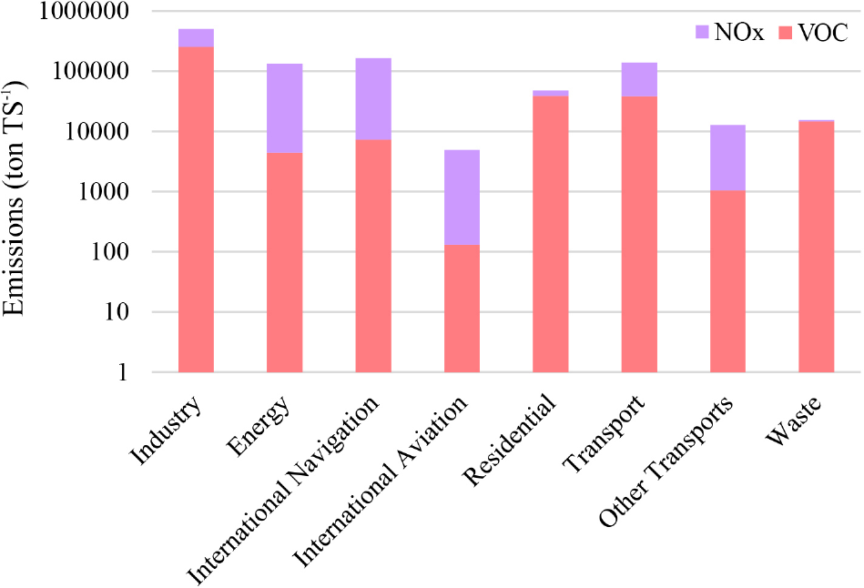
In relation to transportation, with a fleet of approximately 3 million vehicles in the state of Rio de Janeiro, according to INEA³⁶ considering the road network accounted for in the emissions from EDGAR, this becomes coherent. Figure 8 shows the emissions in tons per time of simulation (TS) for the main pollutants.

Figure 8
Emission of NOx and VOC pollutants in tons. TS^-1 for each modeled sector. TS: time of simulation.

According to Alamos et al.,⁸ in their study in Chile, the emission of VOC from EDGAR is more than double the observed value. According to the authors, this is mainly due to the speciation profiles. The application of profiles containing different configurations, whether from thermal treatment equipment in the industry or types of fuel, ends up generating higher emissions. Since there are no inventories of the industrial sector in the state of Rio de Janeiro, it cannot be confirmed that EDGAR overestimated the emissions from industries. However, a generic profile, like the one used in this study, may lead to higher VOC emissions in the domain.⁸

Madrazo et al.,³⁷ in Cuba, also compared local emissions with EDGAR. In the study, EDGAR also showed that most of the VOC emissions from the industry. However, according to the authors, the model overestimates these emissions, while underestimating emissions from transportation, which may lead to a lower contribution than it should from mobile sources to the overall pollutant emissions.

Emission processor validation

Table 5 presents the emission validation using three statistical metrics commonly applied in air quality model evaluation, for the two pollutants analyzed: NOx and VOCs.

Table 5
Statistical validation of emission data in comparison with the mobile source inventory from INEA

Statistic metrics	VOC	NOx
RMSE / (ton year-1)	6776.334	21570.21
NMB / %	-44.4014	-51.0461
NME / %	44.40138	51.04608

As shown, the model generally underestimated the emissions of both evaluated precursors, with a more pronounced underestimation for NOx. The RMSE value indicates that, for VOCs, the absolute error was on the order of six thousand tons per year compared to the observed data. In the case of NOx, the discrepancy exceeded twenty thousand tons annually, highlighting a significant underestimation by the model.

Regarding bias, an underestimation of over 40% was observed for both pollutants, which is corroborated by the values of the NME. This more pronounced discrepancy in the simulated emissions can be attributed mainly to the low spatial resolution of the EDGAR inventory, which fails to adequately represent secondary urban roads within the study area. As a result, vehicular emissions tend to be underestimated, particularly in densely urbanized regions.

Despite the model’s limited performance in terms of accuracy, its application remains relevant, especially in light of the absence of detailed regional emission inventories for the state of Rio de Janeiro. The lack of observational data for several sectors makes it impossible to incorporate real-world information into the modeling process, rendering the global EDGAR inventory an essential tool for air quality simulations.

Moreover, due to the unavailability of sector-specific data for industry, power generation, maritime and air transport, solid waste, and the residential sector, it was not possible to validate emissions from these sources. Nevertheless, these sectors are potential sources of important precursors that significantly influence the formation and dynamics of tropospheric ozone in the study region, reinforcing the need for their inclusion-even if based on global estimates.

Comparison between model data and inventory data

For the comparison of the data, emission values from the mobile source inventory for the metropolitan region of Rio de Janeiro, conducted by INEA in 2013, were used. For the other sectors, there are no official emission inventory data available. Therefore, the comparison will be made only with the transportation sector data from EDGAR.

It is worth noting that the inventory from the managing agency is based on emission factor estimates calculated rather than measured data. This method may be more conservative, which could result in overestimated values compared to reality. Figure 9 shows the emissions from the transportation sector of the global model allocated spatially, with the road network inventoried by INEA shown in the lower-right corner.

Figure 9
Adapted image with main roads allocated by the SMOKE emission processor using EDGAR data in comparison with the roads mapped by the INEA inventory base year 2013.

As can be observed in the EDGAR figure, the metropolitan region of Rio de Janeiro exhibits an emission concentration closely aligned with the road network presented in the inventory prepared by INEA. Therefore, the location of the data generated by the model closely reflects the real-world scenario.

For comparison purposes, the emission data from mobile sources in 2013 were linearly extrapolated based on the increase in the vehicle fleet over the years. This resulted in a 22.23% increase in the fleet size from 2013 to 2018. The calculation of this percentage was based on the growth of the fleet in the city of Rio de Janeiro during this 5-year period, considering the total number of vehicles, a value close to that found in the study conducted by the National Confederation of Municipalities.³¹ This value was then applied to the pollutant emission values. Furthermore, since the modeled emissions align with the simulation period, they were also extrapolated for one year to allow for comparison. This was done by simply multiplying the emissions by 12 months. To mitigate potential errors from the linear fleet projection, three distinct fleet increase scenarios were calculated: one representing the increase in the state identical to the city of Rio de Janeiro, the second considering a lower increase in emissions due to technological advancements and fleet age changes, and the third, a more pessimistic scenario with higher emissions proportional to the fleet increase. Table 6 presents the comparison between the report data and those generated by the SMOKE processor.

Table 6
Comparison between observed and modeled emission data of the main pollutants

Emissions scenario	NOx / (ton year-1)	VOC / (ton year-1)
INEA (2013)	42256.34	15261.54
INEA-22%	51649.92	18654.18
INEA-12%	47424.29	17128.03
INEA-32%	55875.56	20180.33
EDGAR (2018)	20686.13	8485.206

As can be observed, the model underestimates the emissions of both compounds in the region, with modeled values being 38.3 and 48% lower than the observed values for NOx and VOC, respectively. This can primarily be attributed to the lower coverage of traffic lanes or the lower resolution of the model compared to real data. The simulated scenario that most closely aligns with reality is the one with a 17% increase, a smaller increment. This may also be due to the general underestimation produced by EDGAR. Another possibility is the overestimation in the inventory from the managing agency, as it is also based on emission factors and estimates of circulating fleet, fleet age, etc.

Chen et al.³⁸ showed that even with increments, EDGAR underestimates emissions from the transport sector. In their study, the authors found a difference of approximately 200 tons year^-1 for NOx and 50 tons year^-1 for VOCs. This difference is much smaller than the one found in the present study, which may be related to the increment applied to these pollutants in the referenced study.³⁸

In contrast, Lekaki et al.⁷ found that there has been a decrease in emissions across the Americas; however, for NOx, Brazil remains the fifth-largest contributor to the global inventory. The country shows periods of both increases and decreases in emissions, with an average difference of 29%, over the period from 1990 to 2016, a typical behavior observed in countries within the HTAP data.⁷

Puliafito et al.¹⁵ showed that EDGAR likely underestimated emissions from mobile sources in Argentina, primarily due to the significant presence of natural gas-powered cars, a local peculiarity that may not have been adequately specified. Another possibility for the underrepresentation of VOCs in this study is that the fuel characteristics in the state of Rio de Janeiro differ significantly from those in São Paulo or the rest of the country. The presence of CNG (compressed natural gas) in the Rio de Janeiro vehicle fleet results in a higher percentage of aldehydes in emissions, a proportion much lower when observing the vehicle fleet in São Paulo. Thus, a fleet profile derived from São Paulo may reduce the percentage of this organic class in the simulated emissions for Rio de Janeiro. Puliafito et al.³⁹ found that when comparing Argentina’s specific emission inventory with that of EDGAR, the agreement was only 10 and 23% for NOx and VOCs, respectively. These differences are primarily due to EDGAR applying emissions to primary and secondary roads, where lower-tier roads are not as detailed compared to the inventory in the study. This distinct distribution results in emission discrepancies. This same phenomenon can be observed in the present study, where arterial roads in the metropolitan region of Rio de Janeiro are not as detailed in EDGAR.

Influence of the chemical profiles on the model’s emissions

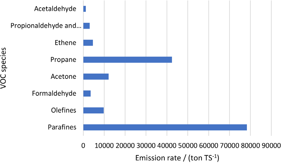
The analysis of the species of interest is primarily focused on the total mass of each species and their percentages within the VOC class as a whole. Paraffins and olefins, species that are abundant in the study area, both show values exceeding 90,000 tons across the entire domain of the study. These species are mainly associated with mobile sources due to the fuels used, fixed sources, primarily from the chemical industry, and various types of combustion of petroleum-derived fuels, such as cooking processes. Figure 10 presents the total emissions of the selected organic species of interest based on the chemical profiles provided.

Figure 10
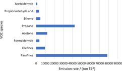
Total emissions of the species of interest from the VOC chemical profiles over the simulation period.

Figure 11 presents the contributions of each species of interest to the total VOC emissions in the simulated domain. The total VOC emissions are significantly higher compared to the percentages of the species of interest. This is due to the variety of species included in the profiles.

Figure 11
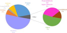
Percentage of each species of interest in the total VOC emissions for the entire domain over the simulation period.

In Figure 11, it can be observed that, as seen in the profiles, the VOCs of interest that contribute the most to the emissions are paraffins. However, these paraffins account for only 21.94% of the total VOC emissions in the simulation domain, indicating that there is a wide variety of VOCs present in the domain.

The high percentage of paraffins represents the significant contribution of petroleum-derived products in the emission profile of the location. Additionally, the explicit inclusion of propane in the chemical mechanism makes it more prominent in the profiles, which aligns with the greater contribution of the residential, transportation, and industrial sectors to the total VOC emissions.

Li et al.¹⁸ also showed in their speciation of certain industrial sectors in China that for the steel and energy sectors, the main compounds belonging to these sectors are alkanes, with about 11 and 19% of their mass composed of ethanes and 3 and 2% of propanes, respectively. The other 27 compounds are also alkanes. The same conclusions are found by Na et al.⁴⁰ in South Korea, where ethane and propane make up the majority of VOC emissions from the transportation sector.

Allen et al.⁴¹ showed that the presence of cooling and heating equipment in the chemical industry sector, such as cooling towers and flares, results in significant quantities of higher olefins, ethene, and propene during their processes. Since the industrial sector is the largest contributor to VOC emissions in the domain of the present study, the lower representation of these compounds may be linked to the generic chemical profile used for the industrial sector.

Dominutti et al.²⁹ in their study of air quality in São Paulo, showed a high concentration of alkanes, mainly ethane and propane, which the authors attribute to the vehicle fleet in the city. Hydrocarbons, along with aldehydes, contribute to ozone formation in the city.

Studies on air quality in the city of Rio de Janeiro and the metropolitan region showed that the most reactive VOCs in the region are alkanes, alkenes, and aromatics, primarily coming from the transportation sector. Among these, substituted aromatics are the largest contributors to ozone formation in the region.³²,⁴²-⁴⁶

These studies compile research on the reactivity scales of VOCs in relation to their dynamics in the troposphere. The reactivity scales can be based on the kinetic reaction coefficient with the OH radical and are determined by box models using simplified meteorology and a robust chemical mechanism. The main scales are: MIR (maximum incremental reactivity), which indicates high sensitivity to VOCs, representing conditions with elevated NOx levels; MOIR (maximum ozone incremental reactivity), which describes conditions more favorable to ozone formation, with lower NOx levels; and EBIR (equal benefit incremental reactivity), which represents conditions with lower NOx, where VOCs and NOx have similar effectiveness in ozone control. These scales help to understand the importance of VOCs for each location, identify which species are most relevant, and analyze their contribution to ozone formation.⁴⁵,⁴⁷ As there are already studies conducted in the studied region, this work will present a discussion on the importance of the species found based on the research already done. Using the MIR scale, Dantas et al.⁴⁵ showed that aromatic compounds and substituted benzene with alkyl groups are the most reactive in the city of Rio de Janeiro. Silva et al.⁴⁴ also using the MIR scale in the city of Rio de Janeiro, showed that aldehydes make a significant contribution to the ozone chemistry in the area.⁴⁴ Geraldino et al.,¹⁹ using the OZIPR model and the MIR scale, showed that alkanes contribute 65-80% to ozone formation in Bangu, Rio de Janeiro. da Silva et al.⁴³ report similar results, showing that alkanes contribute 36-51% in their sampling campaigns. Therefore, the presence of all these species, already referenced in the literature using chemical models and practical tests, is also observed in the mass percentage of VOCs in this study. This demonstrates the good reproducibility of the constructed chemical profile and the emission model for the location being modeled, highlighting a considerable concentration of paraffins and olefins.

The major presence of propane and paraffins in VOC emissions can be associated with the residential profile. In cities in Mexico, where LPG is used, the presence of propane is characteristic.

Conclusions

The study of emissions proved promising, mainly because it presented profiles similar to real-world data and those observed globally, particularly in Latin America. The speciation of VOCs is crucial due to their reactivity and the roles they will play in atmospheric reactions.

Regarding the emission data by sectors, the largest contributors to NOx emissions are industry, international shipping, and energy, accounting for 38, 24, and 19%, respectively. This is primarily due to the presence of three major port terminals located in the northern, metropolitan, and southern regions of Rio de Janeiro. The industries located in the metropolitan and southern regions, as well as some thermoelectric plants operating during the study period, also contribute significantly. For VOCs, the largest contributions came from industries, residences, and transport, at 71, 11, and 11%, respectively. These contributions are mainly due to the combustion of petroleum-derived fuels, which are the primary fuel sources in Brazil.

The comparison with real data shows that the emissions of VOCs and NOx in Rio de Janeiro for the transportation sector are closer to a scenario with a 12% fleet increase, the scenario with the smallest increment. This suggests that the model may have underestimated the emissions of these pollutants for the transportation sector, but not necessarily for other sectors.

Regarding the species of interest, alkanes present the highest mass contribution, primarily due to the main fuel matrix being petroleum. This leads to contributions from both industrial systems and mobile sources. The explicit inclusion of propane in the chemical mechanism and the chemical profile selected during the speciation stage result in its higher presence in the mass of VOCs in the domain. This is mainly due to the selected residential chemical profile and the emissions from the residential sector being one of the three largest contributors for the studied region. However, this does not necessarily represent the real emissions profile.

Therefore, it can be concluded that although the modeled emissions are overestimated, the presence of VOCs aligns with the reality and profile of the study area. This highlights the need for an analysis of the actual emission data from various sectors contributing to local pollution, as well as a more detailed speciation for different sectors and areas of the state of Rio de Janeiro.

Supplementary Information

Supplementary information is available free of charge at http://jbcs.sbq.org.br as PDF file.

Data Availability Statement

Data supporting the findings of this study are available in the text.

Acknowledgments

This study was financed in part by the Coordenação de Aperfeiçoamento de Pessoal de Nível Superior - Brasil (CAPES) - Finance Code 001. We also thank the Carlos Chagas Filho Foundation for Research Support of the State of Rio de Janeiro through Process No. SEI-260003/006265/2024 - APQ1 and the Process No. SEI- 260003/015478 /2021 - APQ1 for the financial support.

References

• ¹ Seinfield, J. H.; Pandis, S. N.; Atmospheric Chemistry and Physics, 3^rd ed.; Wiley: Hoboken, 2016.
• ² Gao, C.; Gao, W.; Song, K.; Na, H.; Tian, F.; Zhang, S.; Resour., Conserv. Recycl. 2019, 143, 184. [Crossref]
  » Crossref
• ³ Janssens-Maenhout, G.; Crippa, M.; Guizzardi, D.; Dentener, F.; Muntean, M.; Pouliot, G.; Keating, T.; Zhang, Q.; Kurokawa, J.; Wankmüller, R.; Denier van der Gon, H.; Kuenen, J. J. P.; Klimont, Z.; Frost, G.; Darras, S.; Koffi, B.; Li, M.; Atmos. Chem. Phys. 2015, 15, 11411. [Crossref]
  » Crossref
• ⁴ Kawashima, A. B.; Martins, L. D.; Rafee, S. A. A.; Rudke, A. P.; de Morais, M. V.; Martins, J. A.; Environ. Sci. Pollut. Res 2020, 27, 35941. [Crossref]
  » Crossref
• ⁵ Loriato, A. G.; Salvador, N.; Loriato, A. A. B.; Sokolov, A.; Nascimento, A. P.; Ynoue, R. Y.; Moreira, D. M.; Reis, N. C.; Albuquerque, T. T. A.; Rev. Bras. Meteorol. 2018, 33, 521. [Crossref]
  » Crossref
• ⁶ de Souza, C. D. R.; Silva, S. D.; da Silva, M. A. V.; D’Agosto, M. A.; Barboza, A. P.; Energy Policy 2013, 53, 125. [Crossref]
  » Crossref
• ⁷ Lekaki, D.; Kastori, M.; Papadimitriou, G.; Mellios, G.; Guizzardi, D.; Muntean, M.; Crippa, M.; Oreggioni, G.; Ntziachristos, L.; Atmos. Environ 2024, 324, 120422. [Crossref]
  » Crossref
• ⁸ Álamos, N.; Huneeus, N.; Opazo, M.; Osses, M.; Puja, S.; Pantoja, N.; Denier Van Der Gon, H.; Schueftan, A.; Reyes, R.; Calvo, R.; Earth Syst. Sci. Data 2022, 14, 361. [Crossref]
  » Crossref
• ⁹ López-Noreña, A. I.; Berná, L.; Tames, M. F.; Millán, E. N.; Puliafito, S. E.; Fernandez, R. P.; Atmos. Environ. 2022, 269, 118839. [Crossref]
  » Crossref
• ¹⁰ Gómez Peláez, L. M.; Santos, J. M.; de Almeida Albuquerque, T. T.; Reis, N. C.; Andreão, W. L.; de Fátima Andrade, M.; Environ. Sci. Policy 2020, 114, 422. [Crossref]
  » Crossref
• ¹¹ Carvalho, V. S. B.; Freitas, E. D.; Martins, L. D.; Martins, J. A.; Mazzoli, C. R.; Andrade, M. F.; Environ. Sci. Policy 2015, 47, 68. [Crossref]
  » Crossref
• ¹² Centro Nacional da Indústria (CNI); https://perfildaindustria.portaldaindustria.com.br/estado/rj#:~:text=O%20estado%20%C3%A9%20o%20quinto,exporta%C3%, accessed in July 2025.
  » https://perfildaindustria.portaldaindustria.com.br/estado/rj#:~:text=O%20estado%20%C3%A9%20o%20quinto,exporta%C3
• ¹³ Instituto Estadual do Ambiente do Rio de Janeiro (INEA-RJ); Inventário Emissões de Fontes Veiculares Região Metropolitana do Rio de Janeiro Ano-Base 2013, https://www.inea.rj.gov.br/wp-content/uploads/2019/01/Invent%C3%A1rio-de-Emiss%C3%B5es-de-Fontes-Veiculares.pdf, accessed in July 2025.
  » https://www.inea.rj.gov.br/wp-content/uploads/2019/01/Invent%C3%A1rio-de-Emiss%C3%B5es-de-Fontes-Veiculares.pdf
• ¹⁴ Maia, R. P.; Baptista, L.; Martins, E. M.; Quim. Nova 2020, 43, 1375. [Crossref]
  » Crossref
• ¹⁵ Puliafito, S. E.; Allende, D. G.; Castesana, P. S.; Ruggeri, M. F.; Heliyon 2017, 3, e00489. [Crossref]
  » Crossref
• ¹⁶ Crippa, M.; Guizzardi, D.; Butler, T.; Keating, T.; Wu, R.; Kaminski, J.; Kuenen, J.; Kurokawa, J.; Chatani, S.; Morikawa, T.; Pouliot, G.; Racine, J.; Moran, M. D.; Klimont, Z.; Manseau, P. M.; Mashayekhi, R.; Henderson, B. H.; Smith, S. J.; Suchyta, H.; Muntean, M.; Solazzo, E.; Banja, M.; Schaaf, E.; Pagani, F.; Woo, J. H.; Kim, J.; Monforti-Ferrario, F.; Pisoni, E.; Zhang, J.; Niemi, D.; Sassi, M.; Ansari, T.; Foley, K.; Earth Syst. Sci. Data 2023, 15, 2667. [Crossref]
  » Crossref
• ¹⁷ Community Modeling and Analysis System Center (CMAS Center); https://www.cmascenter.org/help/documentation.cfm?model=smoke&version=5.1, accessed in July 2025.
  » https://www.cmascenter.org/help/documentation.cfm?model=smoke&version=5.1
• ¹⁸ Li, G.; Wei, W.; Shao, X.; Nie, L.; Wang, H.; Yan, X.; Zhang, R.; J. Environ. Sci. 2018, 67, 78. [Crossref]
  » Crossref
• ¹⁹ Geraldino, C. G. P.; Arbilla, G.; da Silva, C. M.; Corrêa, S. M.; Martins, E. M.; Environ. Monit. Assess. 2020, 192, 119. [Crossref]
  » Crossref
• ²⁰ Santos, F. S.; Miranda, G. A.; Carvalho, A. N. M.; Carvalho, V. S. B.; de Albuquerque, T. T. A.; Braz. J. Chem. Eng 2019, 36, 775. [Crossref]
  » Crossref
• ²¹ Pattinson, W.; Targino, A. C.; Gibson, M. D.; Krecl, P.; Cipoli, Y.; Sá, V.; Atmos. Environ 2018, 182, 138. [Crossref]
  » Crossref
• ²² ENVIRON International Corporation; Enhanced Meteorological Modeling and Performance Evaluation for Two Texas Ozone Episodes; ENVIRON: Texas, 2001.
• ²³ Meteorological Modeling Performance Guidelines to Replace Old Standards; 10^th Annual Ad-Hoc Meteorological Modelers Meeting (AMMM): North Carolina, 2009.
• ²⁴ Crippa, M.; Guizzardi, D.; Butler, T.; Keating, T.; Wu, R.; Kaminski, J.; Kuenen, J.; Kurokawa, J.; Chatani, S.; Morikawa, T.; Zhang, J.; Pouliot, G.; Racine, J.; Moran, M.; Klimont, Z.; Manseau, P. M.; Mashayekhi, R.; Henderson, B. H.; Smith, S. J.; Suchyta, H.; Muntean, M.; Solazzo, E.; Banja, M.; Schaaf, E.; Pagani, F.; Woo, J.-H.; Kim, J.; Monforti-Ferrario, F.; Pisoni, E.; Niemi, D.; Sassi, M.; Ansari, T.; Foley, K.; The HTAP_v3 Emission Mosaic: Merging Regional and Global Monthly Emissions (2000-2018) to Support Air Quality Modelling and Policies; https://edgar.jrc.ec.europa.eu/dataset_htap_v3, accessed in July 2025.
  » https://edgar.jrc.ec.europa.eu/dataset_htap_v3
• ²⁵ United States Environmental Protection Agency (US EPA); https://www.epa.gov/air-emissions-modeling/speciate, accessed in July 2025.
  » https://www.epa.gov/air-emissions-modeling/speciate
• ²⁶ Empresa de Pesquisa Energética; Balanço Energético Nacional 2022, https://www.epe.gov.br/pt/publicacoes-dados-abertos/publicacoes/balanco-energetico-nacional-2022, accessed in July 2025.
  » https://www.epe.gov.br/pt/publicacoes-dados-abertos/publicacoes/balanco-energetico-nacional-2022
• ²⁷ Sui, C.; de Vos, P.; Stapersma, D.; Visser, K.; Ding, Y.; J. Mar. Sci. Eng. 2020, 8, 588. [Crossref]
  » Crossref
• ²⁸ Luis, J. L. J.; Julio, S. F.; Uriel, G. M.; Emmanuel, G. O.; Atmos. Environ 2003, 37, 2327. [Crossref]
  » Crossref
• ²⁹ Dominutti, P.; Nogueira, T.; Fornaro, A.; Borbon, A.; Sci. Total Environ 2020, 738, 139790. [Crossref]
  » Crossref
• ³⁰ Emery, C.; Liu, Z.; Russell, A. G.; Odman, M. T.; Yarwood, G.; Kumar, N.; J. Air Waste Manage. Assoc. 2017, 67, 582. [Crossref]
  » Crossref
• ³¹ Confederação Nacional dos Municípios; Impacto da Frota de Veículos nos Municípios do Brasil; https://cnm.org.br/storage/biblioteca/2023/Estudos_tecnicos/202309_ET_MOB_Impacto_frota_veiculos.pdf, accessed in July 2025.
  » https://cnm.org.br/storage/biblioteca/2023/Estudos_tecnicos/202309_ET_MOB_Impacto_frota_veiculos.pdf
• ³² Carvalho, J. B. B.; Fortes, J. D. N.; Corrêa, S. M.; Martins, E. M.; Quim. Nova 2020, 43, 870. [Crossref]
  » Crossref
• ³³ McDuffie, E. E.; Smith, S. J.; O’Rourke, P.; Tibrewal, K.; Venkataraman, C.; Marais, E. A.; Zheng, B.; Crippa, M.; Brauer, M.; Martin, R. V.; Earth Syst. Sci. Data 2020, 12, 3413. [Crossref]
  » Crossref
• ³⁴ Rowlinson, M. J.; Carpenter, L. J.; Read, K. A.; Punjabi, S.; Adedeji, A.; Fakes, L.; Lewis, A.; Richmond, B.; Passant, N.; Murrells, T.; Henderson, B.; Bates, K. H.; Helmig, D.; Evans, M. J.; EGUsphere 2023 [Crossref]
  » Crossref
• ³⁵ da Costa, T. F.; Carvalho, J. B. B.; Pedruzzi, R.; Albuquerque, T. T. A.; Martins, E. M.; J. Braz. Chem. Soc 2024, 35, e-20240042. [Crossref]
  » Crossref
• ³⁶ Instituto Estadual do Ambiente (INEA); Inventário de Emissões Veiculares Ano-Base 2022; https://www.inea.rj.gov.br/wp-content/uploads/2024/06/Invent%C3%A1rio-de-Emiss%C3%B5es-Veiculares-Ano-Base-2022-final_ok.pdf, accessed in July 2025.
  » https://www.inea.rj.gov.br/wp-content/uploads/2024/06/Invent%C3%A1rio-de-Emiss%C3%B5es-Veiculares-Ano-Base-2022-final_ok.pdf
• ³⁷ Madrazo, J.; Clappier, A.; Belalcazar, L. C.; Cuesta, O.; Contreras, H.; Golay, F.; Sci. Total Environ. 2018, 631-632, 934. [Crossref]
  » Crossref
• ³⁸ Chen, K.; Wang, P.; Zhao, H.; Wang, P.; Gao, A.; Myllyvirta, L.; Zhang, H.; Atmos. Environ. 2021, 246, 118087. [Crossref]
  » Crossref
• ³⁹ Puliafito, S. E.; Bolanõ-Ortiz, T. R.; Fernandez, R. P.; Berná, L. L.; Pascual-Flores, R. M.; Urquiza, J.; López-Norenã, A. I.; Tames, M. F.; Earth Syst. Sci. Data 2021, 13, 5027. [Crossref]
  » Crossref
• ⁴⁰ Na, K.; Kim, Y. P.; Moon, I.; Moon, K. C.; Chemosphere 2004, 55, 585. [Crossref]
  » Crossref
• ⁴¹ Allen, D.; Murphy, C.; Kimura, Y.; Vizuete, W.; Edgar, T.; Jeffries, H.; Kim, B.-U.; Webster, M.; Symons, M.; https://gaftp.epa.gov/Air/nei/ei_conference/EI13/uncertainty/allen.pdf, accessed in July 2025.
  » https://gaftp.epa.gov/Air/nei/ei_conference/EI13/uncertainty/allen.pdf
• ⁴² Mendes, D.; Dantas, G.; da Silva, M. A.; de Seixas, E. G.; da Silva, C. M.; Arbilla, G.; Bull. Environ. Contam. Toxicol 2020, 104, 438. [Crossref]
  » Crossref
• ⁴³ da Silva, C. M.; Corrêa, S. M.; Arbilla, G.; Bull. Environ. Contam. Toxicol. 2018, 100, 184. [Crossref]
  » Crossref
• ⁴⁴ da Silva, C. M.; da Silva, L. L.; Corrêa, S. M.; Arbilla, G.; Rev. Virtual Quim. 2017, 9, 1887. [Crossref]
  » Crossref
• ⁴⁵ Dantas, G.; Siciliano, B.; da Silva, C. M.; Arbilla, G.; Atmos. Pollut. Res. 2020, 11, 1018. [Crossref]
  » Crossref
• ⁴⁶ da Silveira, V. R.; de Oliveira, J. F.; da Silva, M. S.; Silva, C.; Alves, A. R.; de Souza Pontes, A.; Pimentel, L. C. G.; Filho, O. C. R.; Land Use Policy 2021, 101, 105148. [Crossref]
  » Crossref
• ⁴⁷ Oliveira, R. L.; Custódio, D. J.; de Rainho, C. R.; Morais, E.; Felzenszwalb, I.; Corrêa, S. M.; Azevedo, D. A.; Arbilla, G.; Air Qual. Atmos. Health 2018, 11, 581. [Crossref]
  » Crossref

Edited by

• Editor handled this article:
  Maria Cristina Canela (Associate)

Publication Dates

• Publication in this collection
  29 Aug 2025
• Date of issue
  2025

History

• Received
  21 Apr 2025
• Accepted
  29 July 2025