Deep Learning for Optimizing Microwave Resonator Design
Abstract
The article presents a design optimization method for microwave resonators. This method is based on the development of an artificial neural network (ANN) to calculate the physical parameters of resonators used in microwave resonators, which results in resonator characteristics according to the operating frequency requirements of the design. The proposed approach uses a resonator with a T-inverted geometry as the basis for modeling and validating the artificial neural network. The designed resonator is manufactured and measured according to the physical parameters provided by the network. The results obtained from the simulations of the resonator designed by the proposed method and the measurements show good agreement. For the provided examples, the prediction error of the model reaches 2.55%, indicating an accuracy of over 97%, confirming the validity of the proposed approach.
Index Terms
Artificial neural network; design optimization; microwave resonators; T-inverted geometry.
I INTRODUCTION
The design of microwave structures typically relies on theoretical calculations and electromagnetic (EM) simulations to establish the physical parameters needed for specific electrical performance goals. This process, however, can be time-intensive, especially as the complexity of the resonator increases. Each adjustment to a parameter necessitates a new EM simulation, which extends the time required to achieve the desired outcomes. Additionally, if the device needs to be reconfigured for different frequency bands or applications, the entire calculation and simulation process must be repeated, further increasing the time and resources involved [1].
In recent years, Machine Learning (ML) techniques, particularly Artificial Neural Networks (ANNs) and evolutionary optimization algorithms, have emerged as valuable tools in the field of electromagnetic modeling and microwave component design [2]. ANNs, for instance, are capable of learning the relationship between geometrical variables and the EM response of a microwave resonator through a training process that involves multiple simulations. This capability allows ANNs to make accurate and rapid predictions of the EM behavior of microwave components based on their geometric parameters, which is highly beneficial for high-level circuit system design [3], [4], [5].
Among the various types of neural networks, the multilayer perceptron (MLP) is particularly noteworthy for its widespread use in microwave design applications, such as in healthcare systems [6] and the analysis of microwaves absorption [7]. The MLP's well-established error-backpropagation training algorithm and ease of implementation make it a popular choice for modeling and parameter optimization of microwave resonators. Since the MLP is a black-box model that relies on the model’s architecture, hyperparameters and training data, both in terms of size and quality, to obtain optimum desired performance and high accuracy. In microwave design, this data is typically obtained via EM simulations or physical measurements of the components [8].
By leveraging MLPs in the optimization process, designers can significantly reduce the time and computational resources required compared to traditional methods. The ability of MLPs to efficiently model and predict the behavior of microwave resonators makes them an essential tool in the modern design and optimization of these components [9].
This work presents an MLP neural network designed to determine the physical dimensions of a planar resonator based on the desired frequency response. With this approach, users can obtain the necessary physical parameters to achieve the desired resonator response without needing to perform optimization using electromagnetic simulation software. An example resonator is synthesized using an ANN to calculate the physical parameters of the resonator so that the resonator operates at the desired frequency. The resonator response was simulated in Ansys Electronics, the resonator was manufactured, and its frequency response was measured.
The proposed method fits within the category of electromagnetic inverse modeling using surrogate models, specifically artificial intelligence-based approaches. As discussed by [10], such techniques offer efficient solutions for nonlinear problems in resonators design.
II RESONATOR DESIGN AND DATA GENERATION
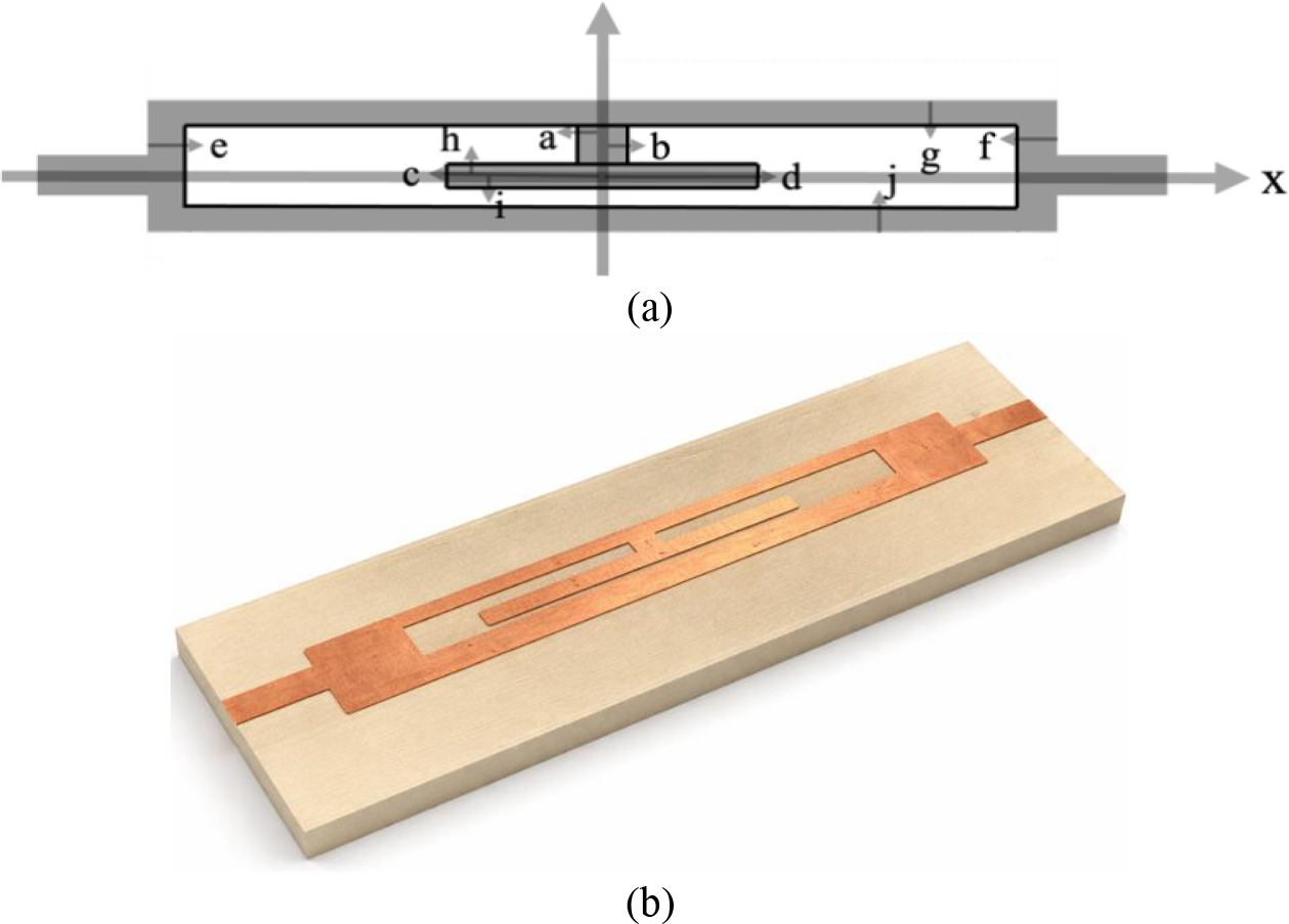
A T-inverted geometry resonator is designed as the basis for an MLP to optimize the resonator design for a target frequency. It uses an RO3010 substrate (Rogers Corporation®) with h = 1.27 mm, ɛr = 10.2, and a loss tangent of 0.0022. The resonator is 10 mm wide, 40 mm long, and operates from 1 GHz to 2.6 GHz, rejecting interference in this range, ideal for radar systems by enhancing signal clarity and accuracy. Its central frequency is adjustable to specific needs. The power line has a 50 Ω impedance and a 1 mm width.
The resonator is implemented as a planar microstrip structure. All gray regions shown in Fig. 1(a) correspond to copper metallization printed on the top surface of the RO3010 substrate, while the bottom layer consists of a continuous ground plane. The inverted-T element located at the center is electrically connected to the upper horizontal arm, forming a single conductive structure.
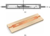
From a 2D point of view, the resonator is made up of a set of 10 variables: a, b, c, d, e, f, g, h, i, e j, which correspond to specific lengths within the resonator structure as shown in Fig. 1. By manipulating and adjusting the size of these dimensions, it is possible to change the resonator's frequency response, bandwidth and other performance parameters.
To generate data for training, validation, and testing, simulations were performed to analyze the resonator's response as each parameter varied over the values in Table I, with the others held constant. The frequency response was measured by S21 from 0 to 4 GHz, with a 4 MHz resolution. This dataset was generated using full-wave 3D electromagnetic simulations performed in Ansys HFSS (finite element method). A parametric sweep was conducted by varying the ten geometrical parameters within the ranges specified in Table I.
Each simulation produced the corresponding S21 response from 0 to 4 GHz with 4 MHz resolution. The resulting dataset consisted entirely of simulated data. The fabricated prototype was used exclusively for validation of the trained model.
III PROPOSED MLP MODEL AND PARAMETERS
The proposed inverse model uses as input the desired magnitude response of S21 (|S21| in dB) over the frequency range of interest. Therefore, the network receives the designer-defined target transmission response and outputs the corresponding geometric parameters required to achieve it.
Only the magnitude of S21 was considered in this work. The reflection coefficient S11 was not included, since the primary objective was to control the resonant frequency and attenuation level at resonance. The other dimensions, including substrate length, height, and dielectric constant, remain constant.
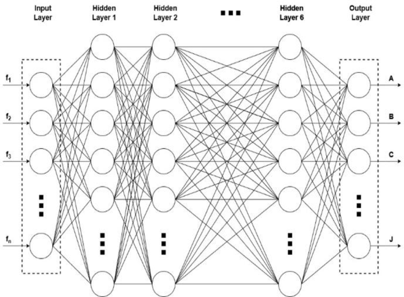
The proposed model (Fig. 2) consists of 8 layers: an input layer, six hidden layers and an output layer, with each of the hidden layers containing six hundred neurons. The first two and the last two hidden layers use the hyperbolic tangent activation function (tanh), which is effective for zero-centered data, while the intermediate layers use ReLU (Rectified Linear Unit), which helps avoid gradient problems and accelerates learning.
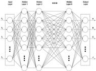
The input vector consists of 200 uniformly sampled points of the magnitude of S21 (in dB), corresponding to a 20 MHz resolution over the 0-4 GHz range. Only the magnitude response is used, and no complex-valued representation (magnitude and phase) is considered. All input features are normalized between -1 and 1 prior to training.
The loss function used is Mean Absolute Error (MAE), which is robust to outliers and suitable for regression problems. The optimizer chosen is Adam (Adaptive Moment Estimation), which dynamically adjusts the learning rates, combining the benefits of other optimization methods: AdaGrad and RMSProp. It adjusts the learning rates based on estimation of the first and second order moments (mean and variance of the gradients), providing faster and more stable convergence.
It is important to note that the MLP does not receive only scalar parameters such as central frequency or return loss. Instead, the full spectral response of S21, represented by 200 sampled points, is used as input. The mention of central frequency and attenuation refers only to the definition of target responses, not to the input dimensionality of the network.
IV TRAINING AND VALIDATION
Only 20% of the total input variables available in the dataset were selected as MLP inputs to optimize the training process and prevent excessively large network architectures. This selection resulted in 200 input features, corresponding to a frequency resolution of approximately 20 MHz over a range of 0 GHz to 4 GHz.
Afterward, the reduced dataset was randomized and divided into three subsets: training (60%), validation (20%), and testing (20%). This division is crucial for developing a robust model. The original S21 responses were obtained with a frequency resolution of 4 MHz over the 0-4 GHz range. To reduce input dimensionality and computational cost, uniform down sampling was applied, resulting in 200 input features corresponding to a 20 MHz resolution. This reduction preserves the essential spectral behavior while improving training efficiency.
The training set is used to adjust the model’s parameters by learning patterns from the data. The validation set aids in fine-tuning hyperparameters and preventing overfitting by assessing the model’s performance on unseen data during training. Lastly, the test set provides an unbiased evaluation of the model’s generalization ability on completely new data, ensuring reliable performance in real-world applications.
Furthermore, to enhance training efficiency and stabilize weight updates, both training and validation data are further divided into batches of size 100.
The MLP was implemented in Python using a neural network framework for training and optimization. Training was performed on a workstation equipped with a multi-core CPU (Intel i7 class), 16 GB of RAM, and an NVIDIA RTX-class GPU.
Several architectures were evaluated during preliminary experiments, including networks with 4, 6, 8, 10, and 12 layers. Networks with fewer than 6 layers exhibited underfitting behavior, while deeper architectures (>10 layers) increased computational cost without significant improvement in validation error and showed early signs of overfitting. The selected 8-layer configuration provided the best trade-off between prediction accuracy, training stability, and computational efficiency.
V RESULTS AND ANALYSIS
The neural network's performance was evaluated on the test dataset using four key metrics: Mean Absolute Error (MAE), Mean Absolute Percentage Error (MAPE), Root Mean Squared Error (RMSE), and R-squared (R2). MAE represents the average absolute difference between predicted and actual values, while MAPE expresses this error as a percentage, aiding interpretation across different scales. RMSE, by squaring errors before averaging and taking the square root, gives more weight to larger errors, making it more sensitive to outliers. R2 (coefficient of determination) measures how well the model explains data variability, ranging from 0 to 1, with higher values indicating better performance, though negative values suggest poor fit. Table I presents these results, providing a detailed analysis of the model’s accuracy and generalization.
The results show varying performance across outputs. Parameters c, d, e, f, g, i, and j achieve the best results, with lower MAE, MAPE, and RMSE values and higher R2 scores. Conversely, parameters a and h exhibit higher errors and negative R2, indicating less accurate predictions.
Table II shows some examples of the physical parameters (mm) obtained according to the requested operating frequency. Following this, the resonator simulation was performed using the parameters obtained for each desired frequency.
The results simulation, including the comparison between the desired operating frequency and the frequency obtained in the simulated results, are presented in Table III.
To validate the proposed approach with the proposed model in obtaining the physical parameters of the resonators, a resonator was synthesized based on the network's predictions. Initially, the MLP was used to estimate the resonator parameters according to the desired frequency, which was defined as:
● Central frequency: f0,ANN = 1.65 GHz
● Return loss: S21,ANN = -25 dB;
As a result, the network provided the following parameters: a = -0.69344; b = 0.678085; c = -8.04078; d = 7.5156; e = -10.9297; f = 10.9027; g=0.828067; h = 0.287038; i = -0.422082; j = -0.597781.
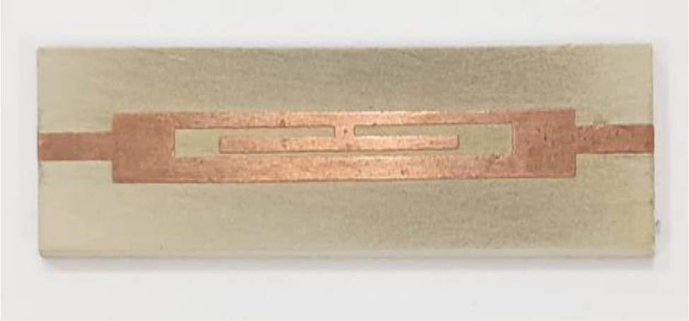
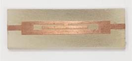
In terms of simulation efficiency, the 3D electromagnetic simulation software required approximately 14 minutes to find the desired solution in the test setup. In contrast, the neural network took around 4 hours to train but was then able to find the optimal dimensions for the target frequency in just 7 seconds. The obtained parameters were used in the resonator design and simulation, and the device was then fabricated to validate the simulation. Fig. 3 shows the image of the fabricated resonator.
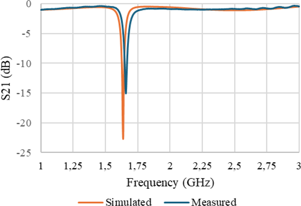
The resonator's frequency response was measured using the Keysight® N9952A vector network analyzer. Fig. 4 presents the simulated and measured frequency response results. For the provided examples, the prediction error of the model reaches 2.55%, indicating an accuracy of over 97%. This confirms that the model is properly adjusted to the measurements, with the predictions in excellent agreement with the actual values.
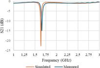
To evaluate the inverse design capability, the desired S21 response was first defined and fed into the trained MLP. The predicted geometrical parameters were then used to perform a new full-wave electromagnetic simulation in HFSS. The curve labeled “Simulated” in Fig. 4 corresponds to this full-wave simulation of the ANN-designed resonator, while the “Measured” curve corresponds to the fabricated prototype.
Once the neural network has been built, the devices can be modeled automatically and accurately, according to the established requirements. The software that uses the trained neural network allows you to enter the center frequency you want to obtain and also the desired magnitude of the S parameter. With this information, the network automatically provides the geometric parameters of the device that meet the specifications.
The overall validation procedure follows an inverse design approach, in which a target S21 response is defined and provided as input to the trained MLP. The network estimates the corresponding geometrical parameters, which are then validated through full-wave electromagnetic simulation. The agreement between the target response, the simulated response, and the measured data confirms the consistency and reliability of the proposed method.
VI. CONCLUSION
Based on an inverted T-resonator, this paper presents an optimization method for microstrip resonator design using an ANN to calculate the resonator's internal dimensions, determining the resonator’s physical dimensions based on the required operating frequency. Numerical results show high accuracy. A resonator with dimensions calculated by the proposed method was fabricated and measured. The MLP model performed excellently for most variables, with accuracy above 90% (MAPE below 10%). Variables "c," "d," "e," "f," "i," and "j" had low MAE and RMSE, with variable "d" achieving an R2 of 0.95, reflecting a great fit. The model provides accurate predictions and, with minor adjustments, can improve performance across all variables. The results show alignment between simulation and measurement, confirming the method’s applicability for designing resonators at desired frequencies. The same network can also be trained to optimize other resonator designs.
DATA AVAILABILITY
The data that support the findings of this study are available from the corresponding author, Araujo, J. A. I., upon reasonable request.
REFERENCES
-
[1] J. A. I. Araujo et al., “Analysis of a microwave filter parameters for design optimization via machine learning,” 2023 SBMO/IEEE MTT-S International Microwave and Optoelectronics Conference (IMOC), IEEE, pp. 100-102, 2023. doi: 10.1109/IMOC57131.2023.10379727.
» https://doi.org/10.1109/IMOC57131.2023.10379727. -
[2] J. Ma et al., “Revolutionizing microwave circuit design with machine learning: challenges and opportunities,” IEEE Communications Magazine, vol. 62, no. 8, pp. 100-106, 2024, doi: 10.1109/MCOM.001.2400209.
» https://doi.org/10.1109/MCOM.001.2400209. -
[3] Lei Zhang, Jianjun Xu, M. C. E. Yagoub, Runtao Ding, and Qi-Jun Zhang, “Efficient analytical formulation and sensitivity analysis of neuro-space mapping for nonlinear microwave device modeling,” IEEE Transactions on Microwave Theory and Techniques, vol. 53, no. 9, pp. 2752-2767, 2005, doi: 10.1109/TMTT.2005.854190.
» https://doi.org/10.1109/TMTT.2005.854190. -
[4] F. Feng, C. Zhang, J. Ma, and Q.-J. Zhang, “Parametric Modeling of EM behavior of microwave components using combined neural networks and pole-residue-based transfer functions,” IEEE Transactions on Microwave Theory and Techniques, vol. 64, no. 1, pp. 60-77, 2016, doi: 10.1109/TMTT.2015.2504099.
» https://doi.org/10.1109/TMTT.2015.2504099. -
[5] J. E. Rayas-Sanchez, “EM-based optimization of microwave circuits using artificial neural networks: the state-of-the-art,” IEEE Transactions on Microwave Theory and Techniques, vol. 52, no. 1, pp. 420-435, 2004, doi: 10.1109/TMTT.2003.820897.
» https://doi.org/10.1109/TMTT.2003.820897. -
[6] A. Singh et al., “Microwave antenna-assisted machine learning: a paradigm shift in non-invasive brain hemorrhage detection,” IEEE Access, vol. 12, pp. 37179-37191, 2024, doi: 10.1109/ACCESS.2024.3371886.
» https://doi.org/10.1109/ACCESS.2024.3371886. -
[7] A. Ahmad et al., “A novel application of mlp networks in classifying l band eco-friendly microwave absorbers,” 2024 IEEE 14th International Conference on Control System, Computing and Engineering (ICCSCE), IEEE, pp. 294-298, 2024. doi: 10.1109/ICCSCE61582.2024.10696895.
» https://doi.org/10.1109/ICCSCE61582.2024.10696895. -
[8] Fang Wang and Qi-Jun Zhang, “Knowledge-based neural models for microwave design,” IEEE Transactions on Microwave Theory and Techniques, vol. 45, no. 12, pp. 2333-2343, 1997, doi: 10.1109/22.643839.
» https://doi.org/10.1109/22.643839. -
[9] A. Uluslu, “Design of microstrip filter by modeling with reduced data,” The Applied Computational Electromagnetics Society Journal (ACES), vol.36, no. 11, pp. 1453-1459, 2021, doi: 10.13052/2021.ACES.J.361109.
» https://doi.org/10.13052/2021.ACES.J.361109. -
[10] H. Kabir, Ying Wang, Ming Yu, and Qi-Jun Zhang, “Neural network inverse modeling and applications to microwave filter design,” IEEE Transactions on Microwave Theory and Techniques, vol. 56, no. 4, pp. 867-879, 2008, doi: 10.1109/TMTT.2008.919078.
» https://doi.org/10.1109/TMTT.2008.919078.
-
Editor:
Carlos E. Capovilla
-
Associate Editor:
Rafael A. Penchel