DMA Master Curves for Long-Term Life Prediction of Epoxy Resins and Composites Using Time Temperature Superposition

Abstract

This study presents the results of constructing the master curve through dynamic mechanical analysis (DMA) of unidirectional composites made of glass fiber and epoxy resins of classes F and H to evaluate the thermal stability and durability of these materials. For this purpose, the viscoelastic behavior of the polymers and composites was evaluated using the time-temperature superposition (TTS) model, applying the empirical Sigmoidal equation and the Williams-Landel-Ferry (WLF) method to estimate the behavior at different temperatures. This approach allows the extension of experimentally accessible frequencies and the description of the entire relaxation behavior of the polymers. The time-temperature shift factor was determined from the DMA curves, generated from individual isotherms at different oscillation frequencies. It was observed that the viscoelastic behavior depends on both frequency and temperature, with a general equivalence between the behavior related to frequency and temperature during the transition processes. The composite materials manufactured by filament winding were also subjected to physical and thermal characterization through differential scanning calorimetry (DSC) and DMA, ensuring the consistent quality of high-performance structural composites. Once the time-temperature shift factors were described by the model, the master curve could be extrapolated to any desired temperature, reducing the need for extensive empirical testing.

Keywords:
Viscoelastic behavior; dynamic mechanical analysis (DMA); master curve; epoxy resins and composites; time-temperature superposition (TTS)

1. Introduction

The thermal class (as F and H) of thermosetting polymers used as a matrix in structural composites refers to the material's behavior when subjected to temperature and exposure time¹. Thermal class refers to the temperature resistance of thermosetting polymers, and they are typically used in the context of electrical insulation materials but can also apply more generally to other thermosetting plastics. Thermosetting polymers are chosen for their ability to resist heat and maintain their shape after curing. The letters "F" and "H" denote the thermal endurance of these materials, where higher letters generally indicate better heat resistance².

Studying the thermal behavior of these materials through the time-temperature superposition principle and thermal properties is the main challenge of this work. This superposition principle is used to determine the mechanical properties of viscoelastic materials that are temperature-dependent, based on known properties at a reference temperature³.

The thermal classification of resins and other insulating materials is essential to determine the suitability of a material for specific applications, especially in environments where heat resistance is critical⁴. These classifications are governed by standards such as IEC 60085, which defines the thermal classes of electrical insulating materials based on the maximum continuous operating temperature. F class resin has an indicated maximum operating temperature of 155°C, offers good thermal resistance, excellent adhesion, and good chemical resistance. H class has a maximum operating temperature of 180°C and is intended for applications where temperatures are even higher⁵.

This study consists of the development of a master curve through DMA of composites made with fiberglass using filament winding and epoxy resin composites of classes F and H. The resins were first subjected to physical and thermal characterization. Subsequently, the samples were then subjected to DMA analysis at different temperatures and frequencies to construct and interpret the master curve, using the empirical Sigmoidal equation⁶. After constructing the master curve, the Williams–Landel–Ferry (WLF) empirical equation was used to estimate the behavior at other temperatures⁷.

The applicability of the master curve, which follows the time-temperature superposition principle, is a fundamental concept in polymer physics. In typical amorphous polymers, elastic moduli increase with the loading rate but decrease with rising temperature. The curves of the instantaneous modulus as a function of time maintain their shape with temperature variations but shift to the left or right⁸. This means that a master curve determined at a specific temperature can serve as a reference to predict behaviors at various temperatures over time, simply by applying a shifting operation⁹.

2. Theorical Background

Time-temperature superposition (TTS) is a principle used to construct master curves. This method assumes that the effects of time (or frequency) and temperature variation are equivalent and can be used to predict the long-term behavior of a material from short-term measurements¹⁰.

Due to their viscoelastic nature, polymers exhibit behavior during deformation that depends on both temperature and time (frequency). This time-dependent behavior suggests that, to accurately assess the material's performance for a given application, it is necessary to test it under the actual temperature and time conditions it will face in its final use¹¹. Fortunately, this type of exhaustive testing is not required. By using accelerated temperature or multifrequency measurements and the theoretical time/temperature superposition of the data, limited laboratory tests (creep, fixed-frequency oscillation, or stress relaxation) are sufficient to design long-term properties under various conditions. The DMA, which measures the modulus (stiffness) and damping properties (energy dissipation) of a material while it is deformed under periodic stress, is one of the best thermal analysis techniques to apply this time/temperature predictive approach¹².

The basis for the time/temperature superposition is the equivalence demonstrated between time (or frequency) and temperature. It has been proven that viscoelastic data collected at a given temperature can be superimposed with data obtained at a different temperature, simply by shifting one of the curves along the time (or frequency) axis¹³.

The principle of superposition is based on the idea that processes related to molecular relaxation or rearrangements occur at faster rates at higher temperatures. The time required for these processes can be reduced by performing measurements at high temperatures and then translating the data to lower temperatures. In this way, the viscoelastic changes that occur quickly at higher temperatures can be adjusted to appear as if they occurred over longer periods or at different frequencies, simply by shifting the data along the time (or frequency) axis¹⁴.

Tan et al.¹⁵ established the master curve of the complex modulus of an asphalt mixture incorporating styrene-butadiene-styrene (SBS) polymer and basalt fiber using the generalized Sigmoidal model. The results indicated that the generalized Sigmoidal model used could better reflect the dynamic mechanical response with accuracy, with correlation coefficients above 0.97, which is used to accurately predict dynamic mechanical performance. Simultaneously, the modulus values showed an increasing trend with loading frequency and a decrease with temperature. However, the phase angle values showed different trends with frequency and temperature.

The performance of bituminous materials was evaluated through rheological properties measured within the linear viscoelastic region by Polacco¹⁶. If there is a unique temperature dependence for all relaxation times, data obtained under different operational conditions can be translated into a logarithmic scale where they partially overlap and merge into a single master curve. According to the author, this is the well-known time-temperature superposition principle. The review summarizes these basic statements along with empirical and phenomenological approaches developed over the years. The aim of the study was to assist the reader in choosing the most suitable method to construct the master curves.

The article published by Virag et al.¹⁷ presents a new approach combining oscillatory shear rheometry techniques and dynamic mechanical analysis to obtain master curves over a wide frequency range. The authors performed finite element analyses to investigate the influence of sample thickness and the Poisson’s ratio on the measured moduli. They demonstrated that the thickness/height ratio of the sample greatly influences its shear stress state. Using polystyrene, which is a simple thermoplastic, the authors determined that continuous master curves can be generated from torsion tests in the molten state and shear tests in the solid state.

According to Jalocha et al.¹⁸, highly filled elastomers exhibit a complex microstructure composed of rigid fillers bounded by a thin-layer polymer matrix. The aim of the work was to analyze the influence of pre-deformation on the viscoelastic behavior and propose a pre-deformation dependent viscoelastic constitutive model. The model is a superposition of three relaxation spectra, each corresponding to a family of polymer chains, and can be considered in its continuous or discrete expression. The analysis was carried out by comparing relaxation experiments and DMA using the relaxation time spectrum. This technique led to models with fewer and more optimal parameters than classical methods based on a logarithmic distribution of relaxation times.

3. Materials and Methods

The epoxy resins used in the experiments were supplied by the company General Electric GE. The F class epoxy resin was manufactured by the company HEXION. The viscosity of the HEXION EPON 828 resin at 25°C is 110 – 150 mPa.s. For the F class resin, the manufacturer recommends a ratio of 100 g of resin to 1.8 g of the CUREZOL 2E4MZ catalyst.

The H class epoxy resin was manufactured by the company Krempel. The viscosity of the KREMPEL DMR 3252 RL resin at 60°C is 2800 – 3600 mPa.s. KREMPEL DMR 3252 RL used a ratio of 100 g of resin to 85 g of the DMH 2112 HL hardening catalyst.

Thermal analysis by DSC was first applied to F and H class epoxy resins, to evaluate the thermal behavior during the curing process. The tests were based on the standard method of ASTM D3418¹⁹. The DSC analysis was conducted using the TA Instruments DSC Q-20 2151 with an RCS40 cooling unit, under a nitrogen atmosphere with a flow rate of 30 mL/min. The test consisted of subjecting a 3 mg of each resin sample, hermetically sealed, to a thermal heating rate of 2°C/min within a temperature range from 25°C to 250°C.

The processing of the composites used a cure cycle of 100°C for 8 hours, followed by 140°C for 10 hours, with a heating ramp of 2°C/min. Due to the high viscosity of the H class resin at room temperature, it was necessary to heat the resin in an oven at 60°C for 4 hours before processing.

The F class resin composites were processed at 120°C for 12 hours, with a heating ramp of 2°C/min. This resin has an appropriate viscosity for processing at room temperature, and no heating process is required for use. The composite composites use fiberglass roving SE1200 1100 as reinforcement. The composites manufacturing was carried out using a Korthfiber filament winding machine, model FW4-CNC, 4 axes, with a feed speed of 2000 mm/min, and fiber orientation at 0°.

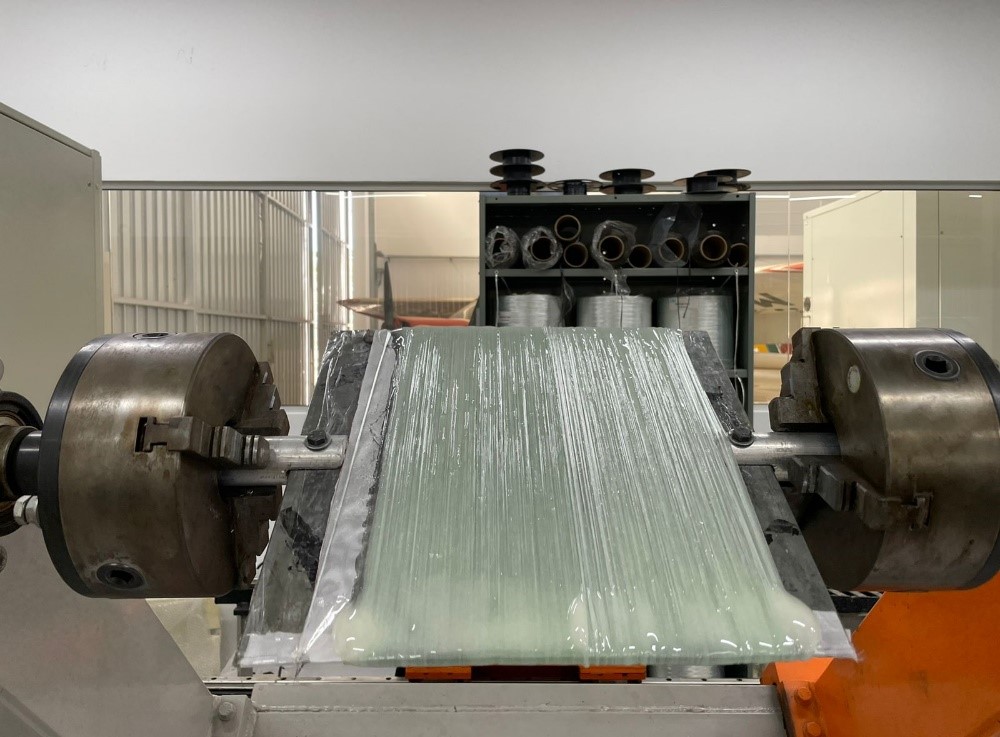
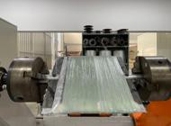
The test specimens were machined according to the ASTM D7028²⁰ and the equipment used for the tests is the DMA SEIKO SII EXSTAR 6000. Peel-ply model A30900 was used on the metal plate and later on the laminate to ensure a smooth surface and good resin distribution throughout the material, as well as to facilitate the demolding process. A21 flat metal plate with dimensions (350x350x2.5 mm) was used as a mold to wrap the fiberglass strand, as shown in Figure 1.

Figure 1
Composite manufacturing by filament winding process.

The samples containing only resin were produced by processing a plate. A flat aluminum plate was used as the mold, with edges defined by Tack Tape to facilitate demolding. The release agent Redelease YCON RDL 40 was applied. After the curing process in the oven, the composites were machined on the CNC Router SHG 1212 to obtain the test specimens.

The WLF equation is commonly used to describe the time/temperature behavior of polymers in the glass transition region. It is based on the assumption that, above the glass transition temperature, the free volume increases linearly with temperature. Additionally, the model assumes that as the free volume of the material increases, its viscosity decreases rapidly¹². The horizontal shift (i.e., in time) required to fit a specific set of data relative to a reference can be mathematically described as a function of temperature. A model frequently used for this is the relationship known as Williams-Landel-Ferry (WLF), represented in Equation 1:

$\log \left(\text{aT}\right)=\frac{-\text{C}1\left(\text{T}-\text{Tr}\right)}{\text{C}2+\left(\text{T}-\text{Tr}\right)}$ (1)

where log(aT) is the base-10 logarithm of the WLF shift factor, T is the temperature, Tr is a reference temperature chosen to construct the master curve of compliance, and C1 and C2 are empirical constants adjusted to fit the values of the superposition parameter aT.

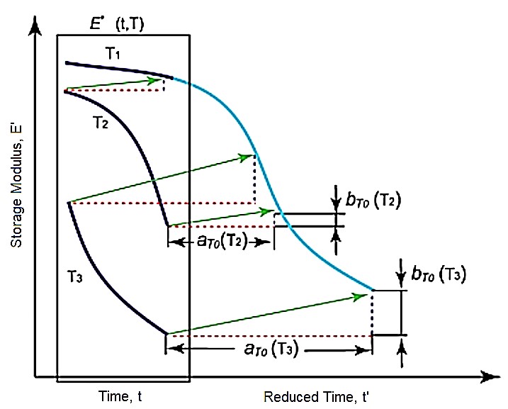
The graph in Figure 2, the vertical axis (Y) represents the storage modulus E’, the horizontal axis (X) shows time on a logarithmic scale and reduced time. The temperatures T1, T2, and T3 are the experimental data collected at different temperatures. The shift factors at0 (T2) and at0 (T3) are horizontally shifted to align with the reference curve. The factors bt0 (T2) and bt0 (T3) are applied to align the amplitudes of the curves.

Figure 2
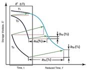
DMA master curve representing the effect of the shift factor. adapted from Cassu and Felisbertini²¹.

The composite and resin samples were tested using the DMA technique through the Exstar SII 6000 equipment, with an oscillation frequency of 1 Hz, amplitude of 10 µm, and a temperature range from 25°C to 250°C, with a heating rate of 5°C/min. The applied force was 4000 mN, aiming to obtain the material's glass transition temperature. The analysis was based on the testing methodology and parameters outlined in the ASTM D7028²⁰. The DMA testing methodology, used to obtain the data for the curve study, was performed in the same way for all materials.

The samples were subjected to 2-minute isothermal tests at different temperatures, with frequency oscillation, in order to obtain data for the construction of the master curve. The Table 1 reveals the test parameters used in the analysis of all the samples, which were subjected to the same conditions.

Table 1
– DMA Master Curve parameters.

Amplitude (µm)	Load (mN)	Frequency (Hz)	Temperature (ºC)
10	4000	0.1	115
		0.5	135
		1	155*
		5	175
		10	195
		25

• ^*
  Tr – Reference Temperature

To obtain the master curve, it was necessary to define a reference temperature value to apply the shift factor (aT), which is used to shift the curves of the isothermal tests, essential for calculating the reduced frequency. The reduced frequency is obtained by multiplying the frequency used in the tests by the shift factor (aT) corresponding to each temperature, and it will be used in the construction of the reference curve.

The Equation 2 was used to calculate the complex modulus E*, obtained from the experiment:

$E^{*}=\sqrt{{\left(E^{\text{'}}\right)}^2+\left(E"\right)²}$ (2)

where E* is the complex modulus, E′ is the storage modulus, and E′′ is the loss modulus.

The complex modulus is a measure of the stiffness of a viscoelastic material and is composed of two components: the storage modulus (E') and the loss modulus (E''). The storage modulus describes the stiffness and the amount of energy stored, while the loss modulus describes the damping behavior (or viscoelasticity) and the energy dissipated.

The Sigmoidal mathematical model was used to construct the master curve, according to the Equation 3:

$\log \left(E^{*}\right)=\delta +\frac{\alpha }{1+e^{\beta }+\log \left(xr\right)}$ (3)

where log (E*) is the logarithm of the predicted complex modulus E*, which is a measure of the stiffness of a viscoelastic material; Delta (δ) is an adjustable parameter that represents a baseline value in the model; Alpha (α) is an adjustable parameter that influences the amplitude of the curve; Beta (β) and Gamma (γ) are adjustable parameters that affect the shape of the curve; Xr is the frequency, an input variable, the reduced frequency of the model.

The reduced frequency is the result of multiplying the test frequency by the shift factor. This technique allows the superposition of experimental data obtained at different temperatures to create a single continuous curve. The adjustable variables (Delta, Alpha, Beta, Gamma) are parameters used in mathematical models to minimize the squared error. By adjusting these variables, the model can be calibrated to better fit the experimental data.

The Excel tool (Solver) is used to fit models to experimental data. These tools allow for complex calculations and testing of multiple hypotheses to find the best fit for the data by analyzing the input variables and the sum of the squared error.

The squared error is the sum of the squares of the differences between the observed values and the values predicted by a model. It is a measure of the model's accuracy, with a smaller squared error indicating a better fit of the data²².

The predicted complex modulus E* is calculated by the sum of the squared error, using adjustable variables Delta (δ), Alpha (α), Beta (β), and Gamma (γ), which are obtained through the Excel software complement (Solver) used to test hypotheses, with the aim of finding an ideal value. To use this tool, it was necessary to calculate the sum of the squared error, which is the subtraction of the complex modulus from the predicted complex modulus raised to a power²³.

The predicted complex modulus E* was calculated using the Sigmoidal model by defining random values for the adjustable variables. Then, the Solver tool was used to obtain the ideal parameters for the adjustable variables Alpha (α), Beta (β), Gamma (γ), and Delta (δ).

The shift factor (aT) is an important concept in the construction of master curves, especially in studies of the viscoelastic behavior of materials. It is used to shift the response curves of a material along the time or frequency axis, allowing for the superposition of experimental data to form a continuous curve. This is done through the application of time-temperature superposition²⁴.

The reference temperature (Tr) is a crucial parameter in the construction of a master curve. It serves as the baseline from which the experimental data are shifted along the time or frequency axis. The choice of the reference temperature can significantly influence the accuracy and usefulness of the master curve. Defining a reference temperature allows for the normalization of results so that they can be compared or combined²⁵.

4. Results and Discussion

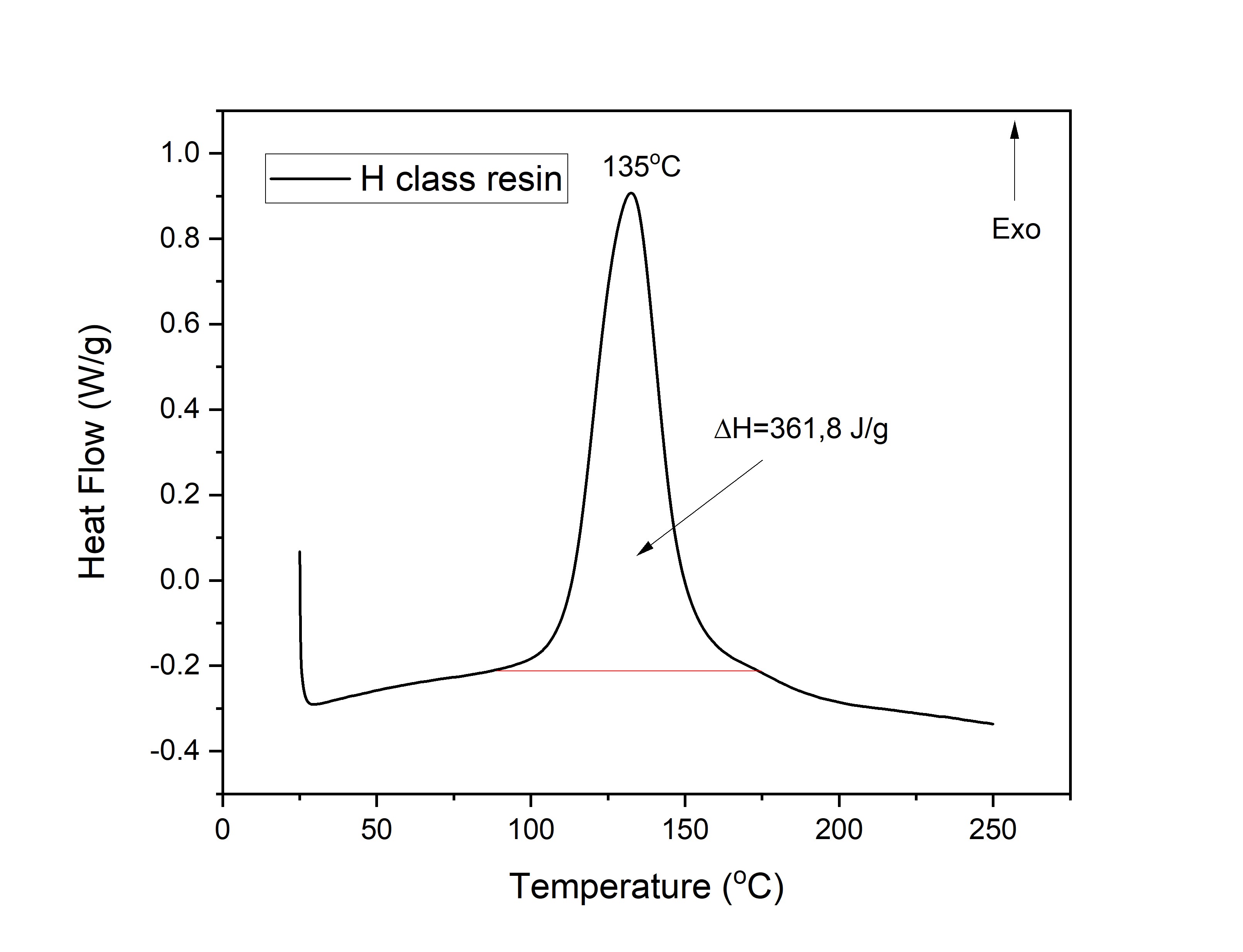
The result of the DSC analysis was able to indicate the main physical phenomena resulting from the applied thermal cycle, such as the curing process of the material. From the DSC curves shown in Figures 3 and 4, it is possible to identify the data related to the enthalpy temperature of the curing process, in relation to the heating rate. For the curing cycle of F class resin, the cure temperature occurs at 109 ºC, and the curing enthalpy (𝛥𝐻) is -374.7 J/g. The H class resin has a cure temperature at 135 ºC, and the curing enthalpy (𝛥𝐻) is -361.8 J/g.

Figure 3
DSC curve for F class resin showing the curing cycle.

Figure 4
DSC curve for H class resin showing the curing cycle.

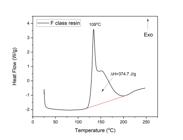
Table 2 presents the results obtained by DMA tests for F class and H class resins and composites at the specified temperatures and frequencies.

Table 2
E’, E’’ and E* obtained from DMA tests.

Temperature (°C)	Frequency (Hz)	F class resin			F Class composite			H Class resin			H Class composite
		E’	E”	E*	E’	E”	E*(GPa)	E’	E”	E*	E’	E”	E*
		(GPa)
115	0.1	25.2	2.0	25.1	116.0	10.9	116.8	33.4	2.7	33.5	145.0	14.9	145.4
	0.5	26.3	2.3	26.5	130.0	15.5	130.6	35.1	2.7	35.2	147.0	15.4	147.5
	1.0	25.1	2.1	25.2	134.0	15.2	134.7	33.6	2.6	33.7	140.0	13.1	140.7
	5.0	26.4	2.3	26.5	132.0	15.9	133.3	35.3	2.7	35.4	144.0	15.7	145.2
	10	27.1	2.4	27.2	131.0	16.8	131.8	36.0	2.9	36.1	147.0	17.4	147.6
	25	27.9	2.7	28.0	130.0	19.0	131.3	36.8	3.2	36.9	147.0	20.4	148.7
135	0.1	15.0	2.7	15.2	111.0	11.5	111.2	23.3	4.8	23.8	90.6	19.4	92.7
	0.5	17.2	2.9	17.2	120.0	10.4	120.4	25.5	5.0	26.0	108.0	20.5	110.0
	1.0	16.2	2.6	16.4	125.0	9.8	125.7	22.1	4.8	22.6	107.0	19.6	108.4
	5.0	18.4	2.9	18.6	128.0	11.3	128.4	25.8	4.9	26.3	107.0	19.5	108.4
	10	19.8	3.1	20.1	128.0	12.1	128.4	27.2	5.0	27.7	116.0	20.6	117.8
	25	20.9	3.1	21.1	127.0	14.7	127.7	29.1	5.3	29.6	126.0	23.2	128.4
155*	0.1	9.2	2.3	9.5	89.2	11.0	89.9	5.1	5.7	7.6	36.8	6.2	37.3
	0.5	11.2	2.6	11.5	98.4	10.2	98.9	6.5	6.8	9.4	42.4	11.6	44.0
	1.0	9.9	2.2	10.1	102.0	10.1	102.4	4.7	4.9	11.0	36.5	5.9	37.0
	5.0	13.1	2.8	13.3	107.0	10.8	107.2	6.3	6.4	12.0	42.2	11.2	43.7
	10	14.3	3.3	14.7	106.0	11.5	106.5	7.6	6.9	13.0	47.1	14.4	49.2
	25	15.6	3.9	16.1	110.0	13.6	110.7	9.1	7.3	15.0	57.0	19.8	60.3
175	0.1	6.7	2.0	7.0	52.8	4.8	53.7	7.4	3.3	4.8	35.5	2.7	29.8
	0.5	8.0	2.7	8.5	98.4	10.0	60.0	4.0	2.9	5.2	36.0	3.6	28.9
	1.0	7.0	1.9	7.2	92.4	9.9	71.5	7.0	2.0	7.4	35.4	2.4	26.4
	5.0	8.4	2.7	8.8	83.7	10.4	72.2	4.3	3.0	5.4	35.9	3.4	31.1
	10	9.2	3.2	9.7	78.2	10.8	79.0	4.2	3.9	5.9	36.3	3.8	36.5
	25	11.0	3.7	11.6	80.7	12.3	81.6	4.0	4.5	6.1	37.1	4.4	32.4
195	0.1	5.2	1.4	5.4	12.6	1.0	8.4	0.8	1.3	1.5	9.6	0.5	19.6
	0.5	5.7	1.7	5.9	11.1	1.0	11.1	0.9	1.6	1.8	7.1	0.8	18.1
	1.0	5.3	1.2	5.4	12.4	0.9	15.4	1.1	1.4	1.8	8.9	0.4	18.9
	5.0	5.8	1.6	6.0	11.1	1.1	20.1	1.1	1.7	2.0	7.0	0.6	19.1
	10	6.1	1.7	6.3	11.0	1.2	23.4	1.0	1.8	2.1	6.9	0.7	17.9
	25	6.5	1.9	6.8	10.8	1.6	26.7	0.8	2.2	2.4	6.7	0.8	18.8

Table 3 presents the values adopted for the change factor (aT) in each sample, using a reference temperature of 155°C for all procedures. By standardizing the reference temperature at 155°C, it was possible to minimize variations arising from temperature differences between the samples, thus facilitating a more direct and comparable analysis of the behaviors of the two resin classes. This approach ensures that any differences observed in the results are mainly attributed to the intrinsic properties of the resins, rather than variations in the test conditions.

Table 3
Determination of the shift fator (aT) at different temperatures.

Sample	Temperature (ºC)	Shift Factor (aT)
F class resin	115	1000000
	135	500
	155	1
	175	0.01
	195	0.0001
F class composite	115	150000
	135	300
	155	1
	175	0.0001
	195	0.0000001
Class resin	115	100000
	135	1000
	155	1
	175	0.001
	195	0.000001
H class composite	115	100000
	135	1000
	155	1
	175	0.001
	195	0.0000009

F class resin shows a very high change factor at lower temperatures (115°C and 135°C), which decreases rapidly as the temperature increases. The F class composite also demonstrates high temperature sensitivity, with a change factor that decreases more drastically than the pure resin. H class resin exhibits a pattern similar to that of F class resin, but with a slightly less drastic variation in the change factor at intermediate temperatures. The H class composite shows behavior similar to the F class composite, but with slightly higher change factors at lower temperatures. All the samples show a decrease in the change factor with the increase in temperature, reflecting the viscoelastic nature of the materials. F class resins and composites tend to have higher change factors at lower temperatures, while H class resins and composites exhibit more stable change factors, although still decreasing with the rise in temperature.

The construction of the master curve was performed using the Sigmoidal mathematical model, presented in Equation 1. Table 4 presents the results obtained when the shift factor was applied as a function of frequency at each test temperature.

Table 4
Values obtained for the predicted complex modulus E* in resins and composites.

Temp. (ºC)	Reduced Frequency (Hz)	F Class resin		F Class composite		H Class resin		H Class composite
		Predicted E*	Square Error	Predicted E*	Square Error	Predicted E*	Square Error	Predicted E*	Square Error
		(GPa)		(GPa)		(GPa)		(GPa)
115	100000	23.75	1.81	126.79	99.84	32.61	0.78	129.34	257.87
	500000	25.16	1.79	128.88	2.94	34.32	0.78	137.00	110.26
	1000000	25.71	0.26	129.68	25.13	34.89	1.41	139.26	2.08
	5000000	26.85	0.12	131.34	3.84	35.92	0.27	142.81	22.92
	10000000	27.30	0.010	131.97	0.02	36.26	0.03	143.81	23.88
	25000000	27.83	0.02	132.73	2.07	36.63	0.07	144.80	182.24
135	50	15.48	0.07	114.80	12.97	18.64	0.13	83.41	86.39
	250	17.31	0.03	118.60	3.21	22.63	0.39	103.06	48.20
	500	18.11	2.94	120.07	31.59	24.28	0.84	110.60	4.85
	2500	19.94	1.80	123.15	27.55	27.78	2.20	124.75	122.15
	5000	20.71	0.37	124.33	16.52	29.11	1.98	129.34	133.21
	12500	21.69	0.35	125.78	3.68	30.67	1.14	134.16	33.22
155	0.1	9.49	0.058	96.31	41.15	6.54	1.13	30.48	46.48
	0.5	10.80	0.48	102.38	12.16	8.24	1.35	35.79	67.43
	1	11.42	1.75	104.78	5.70	9.18	3.32	39.14	4.59
	5	12.99	0.09	109.88	7.18	11.89	0.01	50.27	43.12
	10	13.71	0.96	111.87	28.88	13.28	0.08	56.66	55.61
	25	14.70	1.93	114.33	13.21	15.31	0.09	66.50	38.38
175	0.001	6.81	0.03	49.93	14.20	3.74	1.13	24.48	28.27
	0.005	7.58	0.83	58.97	1.06	4.02	1.39	24.87	16.21
	0.01	7.97	0.59	62.82	75.31	4.19	1.47	25.13	1.60
	0.05	8.99	0.03	71.53	0.44	4.71	0.47	26.08	25.18
	0.1	9.49	0.04	75.15	14.80	5.02	0.78	26.71	95.85
	0.25	10.21	1.91	79.78	3.31	5.52	0.34	27.84	20.82
195	0.00001	5.34	0.002	8.742	0.11	3.29	0.24	24.06	19.89
	0.00005	5.75	0.02	13.48	5.70	3.33	0.02	24.09	35.83
	0.0001	5.96	0.31	15.92	0.27	3.36	0.13	24.10	27.07
	0.0005	6.52	0.27	22.45	5.55	3.44	0.31	24.17	25.67
	0.001	6.81	0.26	25.60	4.87	3.49	0.65	24.21	39.80
	0.0025	7.23	0.18	30.04	11.17	3.57	1.27	24.28	30.08

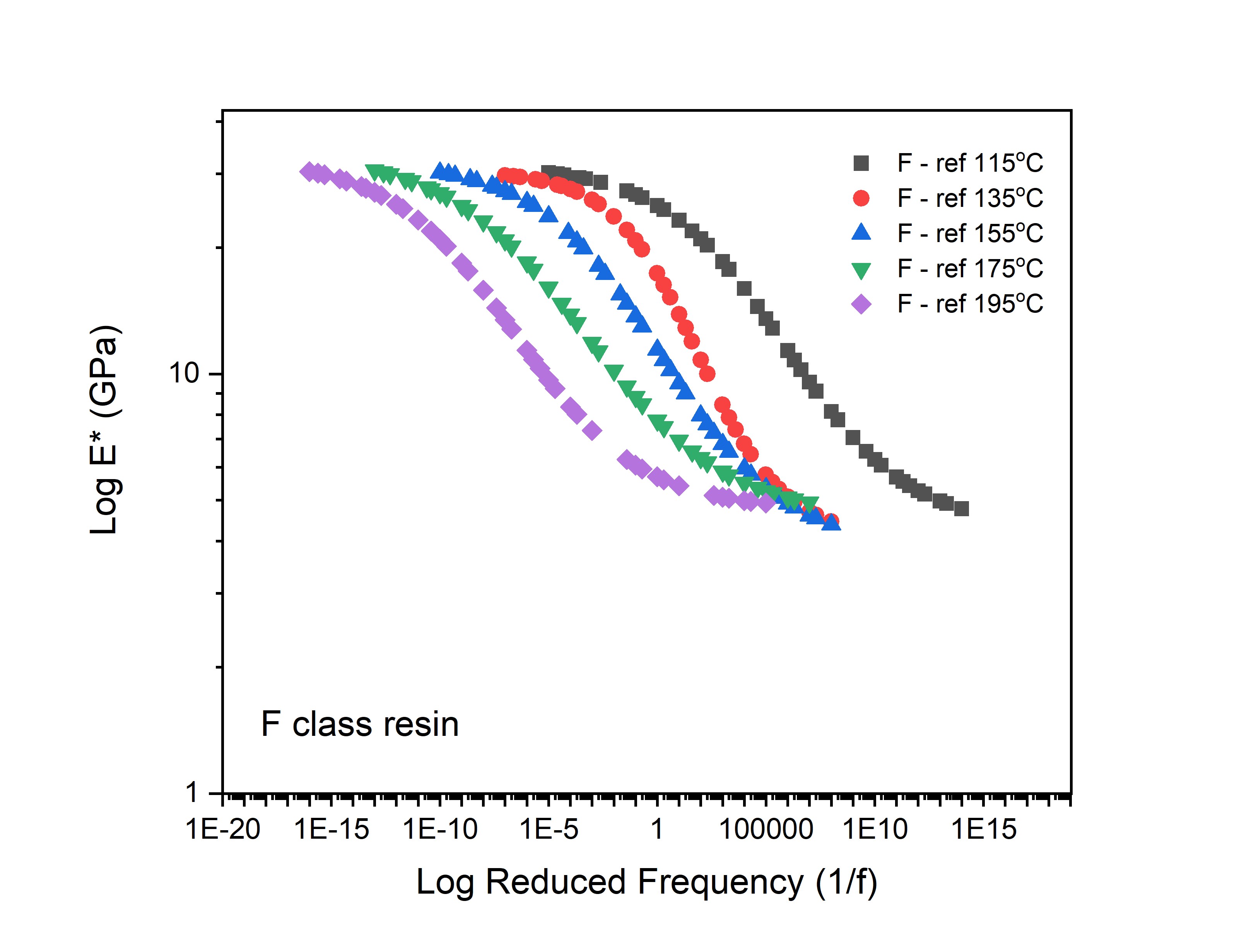
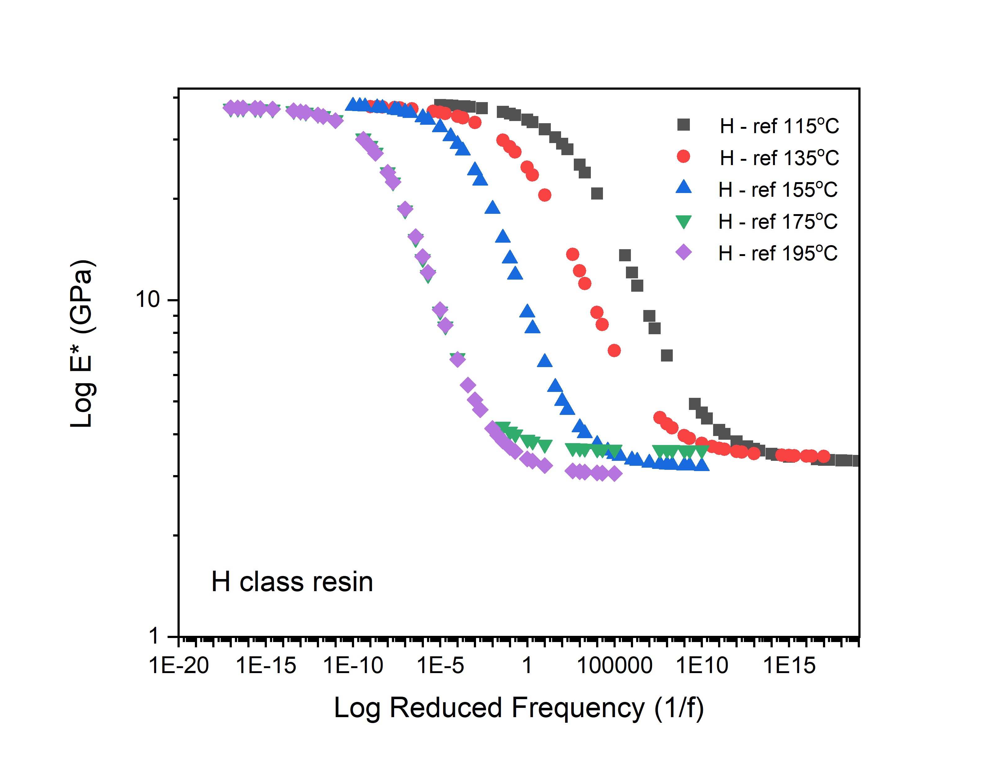
The Figures 5 and 6 represent the curves Log E* vs Log Reduced Frequency obtained by DMA for the F and H class resins at different isotherms (T_iso).

Figure 5
DMA curve for F class resin at different isotherms.

Figure 6
DMA curve for H class resin at different isotherms.

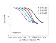
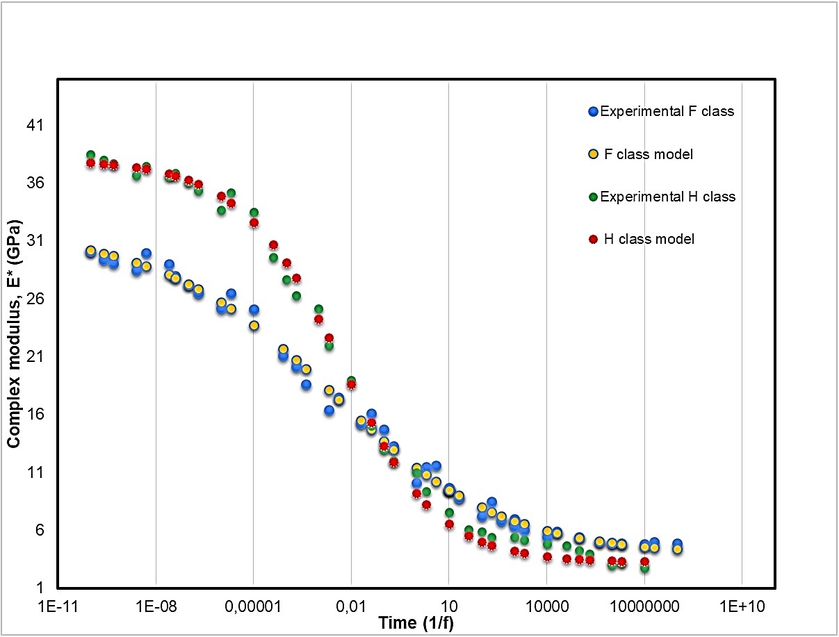
The shift factor is a function that adjusts the experimental data taken at different temperatures (or frequencies) to align onto a single master curve. The shift factor compensates for the temperature (or frequency) dependence of the material's properties. The DMA master curves are presented in Figure 7.

Figure 7
DMA master curves for F and H class resins.

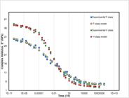
The graph in Figure 7 shows the DMA master curve for the F and H class resins, and it represents the material's viscoelastic properties (such as modulus) across a wide range of frequencies or temperatures, often by shifting data measured at different temperatures to a reference temperature. According to the master curves, it was observed a good correlation between the experimental data and the predicted values for the models. This indicates that the model used is effective in describing the viscoelastic behavior of F and H class resins and composites. The complex modulus decreases as the time increases, for all the materials. This behavior is typical of viscoelastic materials, where the material becomes less rigid as the load application time increases. This decrease is progressive and occurs smoothly.

It can be observed that class H resin has an initial complex modulus higher than class F resin. This resin is more stable at the beginning of the time. At time 0.1, the curves cross at a complex modulus of 16 GPa. From this point onward, class F resin shows a less intense decrease in the complex modulus over time. F class maintains a higher complex modulus than H class throughout the entire time interval, indicating that F class has better thermal stability. It can also be observed that the decrease in the complex modulus occurs more sharply at shorter times, stabilizing as the time increases.

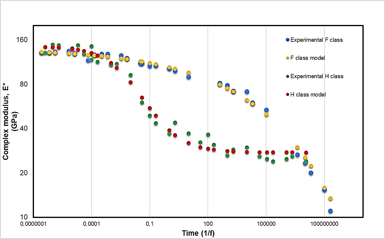
The graph in Figure 8 shows the DMA master curve for the F and H class composites.

Figure 8
DMA master curves for F and H class composites.

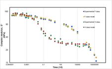
The H class composite has a slightly higher initial complex modulus than the F class composite. This resin shows a sharp decrease in the complex modulus at the beginning of the time, while the F class composite maintains relatively higher stiffness for a longer period. Between times 0.00001 and 0.01, the curves cross at a complex modulus of 115 GPa. From this point onward, the F class composite has a higher complex modulus over time, indicating that it possesses superior stiffness compared to the H class composite. Throughout the entire curve presented, the F class composite shows better thermal stability, with a gradual and smooth loss of the complex modulus, compared to the H class composite, which exhibits a greater loss over time. However, the curves cross again at a complex modulus E* of 25 GPa, where the H class composite maintains a constant modulus, indicating greater thermal stability at longer times.

Table 5 presents the calculated results obtained from the WLF equation for the time-temperature superposition.

Table 5
Values obtained from the WLF equation for the time-temperature behavior of the materials.

Tr (ºC)	aT	Tiso (°C)	F class resin		F class composite		H class resin		H class composite
			Predicted aT	Square Error	Predicted aT	Square Error	Predicted aT	Square Error	Predicted aT	Square Error
115	1000000	75	7.9E+10	6.2E+21	2.0E+12	3.9E+24	8.4E+12	7.1E+25	4.4E+11	1.9E+23
	1000000	80	1.6E+10	2.7E+20	3.4E+11	1.1E+23	1.3E+12	1.7E+24	8.2E+10	6.8E+21
	1000000	85	3.4E+09	1.2E+19	5.7E+10	3.3E+21	2.0E+11	4.2E+22	1.5E+10	2.4E+20
	1000000	90	7.1E+08	5.0E+17	9.7E+09	9.5E+19	3.2E+10	1.0E+21	2.9E+09	8.3E+18
	1000000	95	1.5E+08	2.2E+16	1.7E+09	2.8E+18	5.0E+09	2.5E+19	5.4E+08	2.9E+17
	1000000	100	3.1E+07	8.9E+14	2.8E+08	8.0E+16	7.7E+08	5.9E+17	1.0E+08	1.0E+16
135	500	105	6.4E+06	4.2E+13	4.8E+07	2.3E+15	1.2E+08	1.4E+16	1.9E+07	3.6E+14
	500	110	1.3E+06	1.8E+12	8.2E+06	6.8E+13	1.9E+07	3.5E+14	3.5E+06	1.3E+13
	500	115	2.8E+05	7.8E+10	1.4E+06	2.0E+12	2.9E+06	8.4E+12	6.6E+05	4.4E+11
	500	120	5.8E+04	3.4E+09	2.4E+05	5.7E+10	4.5E+05	2.0E+11	1.2E+05	1.5E+10
	500	125	1.2E+04	1.4E+08	4.1E+04	1.6E+09	7.0E+04	4.8E+09	2.3E+04	5.0E+08
	500	130	2.5E+03	4.2E+06	7.0E+03	4.4E+07	1.1E+04	9.9E+07	4.4E+03	1.1E+07
155	1	135	5.3E+02	2.8E+05	1.2E+03	1.4E+06	1.7E+03	2.9E+06	8.2E+02	6.6E+05
	1	140	1.1E+02	1.2E+04	2.0E+02	4.0E+04	2.7E+02	7.0E+04	1.5E+02	2.3E+04
	1	145	2.3E+01	4.8E+02	3.4E+01	1.1E+03	4.1E+01	1.6E+03	2.9E+01	7.6E+02
	1	150	4.8E+00	1.4E+01	5.9E+00	2.4E+01	6.4E+00	2.9E+01	5.3E+00	1.9E+01
	1	155	1.0E+00	0.0E+00	1.0E+00	0.0E+00	1.0E+00	0.0E+00	1.0E+00	0.0E+00
	1	160	2.1E-01	6.3E-01	1.7E-01	6.9E-01	1.6E-01	7.1E-01	1.9E-01	6.6E-01
175	0,01	165	4.4E-02	1.1E-03	2.9E-02	8.4E-04	2.4E-02	5.4E-04	3.5E-02	1.2E-03
	0,01	170	9.1E-03	8.8E-07	5.0E-03	2.4E-05	3.8E-03	7.7E-06	6.6E-03	3.1E-05
	0,01	175	1.9E-03	6.6E-05	8.4E-04	5.5E-07	5.9E-04	1.7E-07	1.2E-03	5.2E-08
	0,01	180	3.9E-04	9.2E-05	1.4E-04	1.9E-09	9.1E-05	8.3E-07	2.3E-04	5.9E-07
	0,01	185	8.2E-05	9.8E-05	2.5E-05	5.7E-09	1.4E-05	9.7E-07	4.3E-05	9.2E-07
	0,01	190	1.7E-05	1.0E-04	4.2E-06	9.2E-09	2.2E-06	1.0E-06	8.1E-06	9.8E-07
195	0,0001	195	3.6E-06	9.3E-09	7.1E-07	4.9E-13	3.4E-07	4.3E-13	1.5E-06	3.7E-13
	0,0001	190	1.7E-05	6.9E-09	4.2E-06	1.7E-11	2.2E-06	1.5E-12	8.1E-06	5.1E-11
	0,0001	195	3.6E-06	9.3E-09	7.1E-07	4.9E-13	3.4E-07	4.3E-13	1.5E-06	3.7E-13
	0,0001	200	7.4E-07	9.9E-09	1.2E-07	1.2E-14	5.4E-08	9.0E-13	2.8E-07	3.8E-13
	0,0001	205	1.6E-07	1.0E-08	2.1E-08	1.2E-16	8.3E-09	9.8E-13	5.3E-08	7.2E-13
	0,0001	210	3.2E-08	1.0E-08	3.5E-09	4.2E-17	1.3E-09	1.0E-12	9.9E-09	7.9E-13

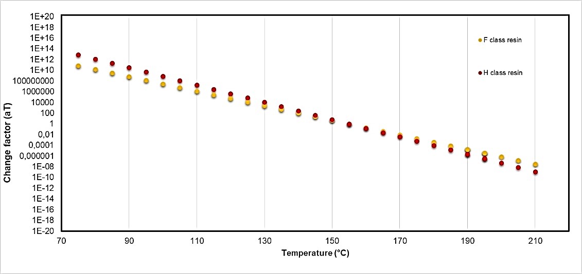
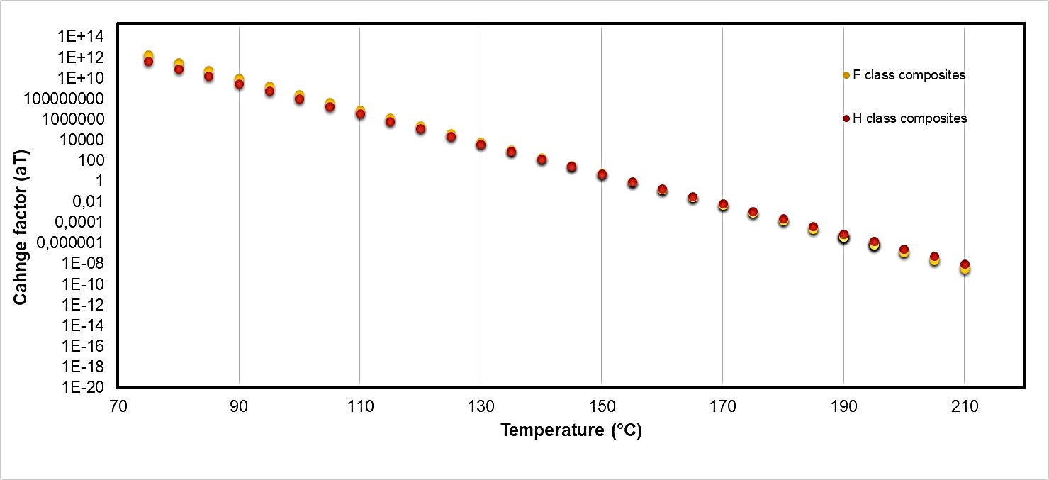
Mean Squared Error (MSE) provides a way to measure the magnitude of error between model predictions and actual values. It is closely related to the variance of the residuals (errors), which represent the difference between predicted and actual values. Therefore, when evaluating the experimental data and quantifying the model performance, it is clear that the models obtained in this study are well adjusted to the experimental data. The data obtained in Table 5 were plotted on a logarithmic scale. The Figures 9 and 10 present the values of aT as a function of the isothermals.

Figure 9
Values of aT as a function of isothermals for F and H class resins.

Figure 10
Values of aT as a function of isothermals for F and H class composites.

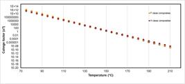
The interpretation of the Figures 9 and 10 allows the construction of master curves of material behavior by shifting data obtained at different temperatures. The shift factor varies exponentially with the inverse of the temperature. Therefore, to predict the behavior of F and H class materials, aT must be identified according to the defined temperature. In practice, the temperature dependence of the shift factor can also be described using empirical or semi-empirical models depending on the specific application.

5. Conclusion

In the DMA results for the resins, it was observed that the glass transition temperature (Tg) of H class resin is higher than that of class F resin. However, when comparing the composite values, the class F composite has a higher Tg than H class, which may indicate a poor fiber/matrix interface.

Class F resin has an initial complex modulus of 26 GPa with an 80% loss over time at the reference temperature. H class resin has a higher complex modulus, 35 GPa, but the loss is greater over time, at 95%. The class F composite has an initial complex modulus of 132 GPa with an 84% loss over time at the reference temperature. The H class composite has a higher complex modulus, 145 GPa, but the loss is slightly greater over time, at 86%.

H class resin on the master curve shows a higher complex modulus than class F resin, but it has a more pronounced loss over time. The empirical and phenomenological approaches developed in this study showed that the master curve reflects the time (in terms of frequency) dependence of the material at a constant reference temperature, T_o. The dependence of the viscoelastic properties on temperature is noted by the variation in the shift factor with temperature.

This study proves that the master curve is a laboratory testing tool that significantly reduces the time and cost for evaluating the thermal stability of polymers and composites. It allows for the prediction of the dynamic-mechanical characteristics of polymeric materials, enabling the extrapolation of a material's behavior at frequencies beyond the measurement range. According to the results, the master curves, based on the sigmoidal empirical equation, Williams-Landy-Ferry (WLF) model and the time-temperature superposition principle, was able to predict the material behavior outside the test temperature range, and it can be used to replace thermal aging tests, which are performed over long periods and can make testing costly.

6. Aknowledgments

The authors acknowledge the financial support from National Council for Scientific and Technological Development (CNPq) under project 303160/2023-3, 407431/2022-5, 447331/2024-8; from Financial Agency for Studies and Projects (FINEP) project number 0.1.13.0169.00, and Fapemig APQ 01846-18. The authors thank the Composite Technology Center (NTC) from the Federal University de Itajubá-Brazil for the general facilities.

7. References

• ¹ Saba N, Jawaid M. The thermal class of thermosetting polymers used as a matrix in structural composites refers to the material’s behavior when subjected to temperature and exposure time. J Ind Eng Chem. 2018;67(2):1-11. http://doi.org/10.1016/j.jiec.2018.06.018
  » http://doi.org/10.1016/j.jiec.2018.06.018
• ² Zhou MH, Yin GZ, Prolongo SG. Review of thermal conductivity in epoxy thermosets and composites: mechanisms, parameters, and filler influences. Adv Ind Eng Polym Res. 2024;7(3):295-308. http://doi.org/10.1016/j.aiepr.2023.08.003
  » http://doi.org/10.1016/j.aiepr.2023.08.003
• ³ Prime RB, Turi EA. Thermal characterization of polymeric materials. San Diego: Academic Press; 1997.
• ⁴ Di Benedetto RM, Janotti AJ, Gomes GF, Ancelotti AC Jr, Botelho EC. Statistical approach to optimize crashworthiness of thermoplastic commingled composites. Mater Today Commun. 2022;31(1):2352-4928. http://doi.org/10.1016/j.mtcomm.2022.103651
  » http://doi.org/10.1016/j.mtcomm.2022.103651
• ⁵ Aziz T, Haq F, Farid A, Cheng L, Chuah LF, Bokhari A, et al. The epoxy resin system: function and role of curing agents. Carbon Lett. 2024;34(1):477-94. http://doi.org/10.1007/s42823-023-00547-7
  » http://doi.org/10.1007/s42823-023-00547-7
• ⁶ Ashter SA. Thermoforming of single and multilayer laminates. Norwich: William Andrew Publishing; 2014. Mechanics of materials; p. 123-45. http://doi.org/10.1016/B978-1-4557-3172-5.00006-2
  » http://doi.org/10.1016/B978-1-4557-3172-5.00006-2
• ⁷ Cheng X, Zhong B, Wu Z. Material-specific coefficients C1 and C2 in Williams-Landel-Ferry equations and phase transition behaviors of asphalt binder reinforced by various basalt fibers. Case Stud Constr Mater. 2024;21:e03619. http://doi.org/10.1016/j.cscm.2024.e03619
  » http://doi.org/10.1016/j.cscm.2024.e03619
• ⁸ Gurvich MR, Andonian AT. On characterization of Williams-Landel-Ferry equation for non-linear analysis. J Mater Sci. 2000;35(2):289-92. http://doi.org/10.1023/A:1004732915037
  » http://doi.org/10.1023/A:1004732915037
• ⁹ Rouleau L, Pirk R, Pluymers B, Desmet W. Characterization and modeling of the viscoelastic behavior of a self-adhesive rubber using dynamic mechanical analysis tests. J Aerosp Technol Manag. 2015;7(2):200-8. http://doi.org/10.5028/jatm.v7i2.474
  » http://doi.org/10.5028/jatm.v7i2.474
• ¹⁰ Ferry JD. Viscoelastic properties of polymers. Hoboken: John Wiley; 1980.
• ¹¹ Souto-Silvar D, Alvarez-García A, Díaz-Díaz A, Rodríguez-Dopico FJ, López-Beceiro J. Application of the time-temperature superposition principle to predict long-term behaviour of an adhesive for use in shipbuilding. Arab J Sci Eng. 2024;49(1):2345-55. http://doi.org/10.1007/s13369-023-08219-4
  » http://doi.org/10.1007/s13369-023-08219-4
• ¹² Landel RF, Nielsen LE. Mechanical properties of polymers and composites. Boca Raton: CRC Press; 1994.
• ¹³ Ferry JD. Viscoelastic properties of polymers. Hoboken: John Wiley & Sons; 1980.
• ¹⁴ Williams ML, Landel RF, Ferry JD. The temperature dependence of relaxation mechanisms in amorphous polymers and other glass-forming liquids. J Am Chem Soc. 1955;77(14):3701-7. http://doi.org/10.1021/ja01619a008
  » http://doi.org/10.1021/ja01619a008
• ¹⁵ Tan G, Wang W, Cheng Y, Wang Y, Zhu Z. Master curve establishment and complex modulus evaluation of sbs-modified asphalt mixture reinforced with basalt fiber based on generalized Sigmoidal model. Polymers. 2020;12(7):1586-94. http://doi.org/10.3390/polym12071586
  » http://doi.org/10.3390/polym12071586
• ¹⁶ Polacco G, Filippi S. Master curves construction for viscoelasticfunctions of bituminous materials. Appl Rheol. 2024;34(1):20-30. http://doi.org/10.1515/arh-2023-0117
  » http://doi.org/10.1515/arh-2023-0117
• ¹⁷ Virag AD, Juhasz Z, Kossa A, Molnar K. Combining oscillatory shear rheometry and dynamic mechanical analysis to obtain wide-frequency master curves. Polymer. 2024;295(1):126-39. http://doi.org/10.1016/j.polymer.2024.126742
  » http://doi.org/10.1016/j.polymer.2024.126742
• ¹⁸ Jalocha D, Constantinescu A, Nevière R. Prestrain-dependent viscosity of a highly filled elastomer: experiments and modeling. Mech Time-Depend Mater. 2015;19(1):243-62. http://doi.org/10.1007/s11043-015-9262-z
  » http://doi.org/10.1007/s11043-015-9262-z
• ¹⁹ ASTM: American Society for Testing and Materials. ASTM D3418-21: standard test method for transition temperatures and enthalpies of fusion and crystallization of polymers by differential scanning calorimetry. West Conshohocken: ASTM; 2021.
• ²⁰ ASTM: American Society for Testing and Materials. ASTM D7028-07: standard test method for glass transition temperature (DMA Tg) of polymer matrix composites by Dynamic Mechanical Analysis (DMA). West Conshohocken: ASTM; 2015.
• ²¹ Cassu SN, Felisbertini MI. Comportamento dinâmico-mecânico e relaxações em polímeros e blendas poliméricas. Quim Nova. 2005;28(2):1-22. http://doi.org/10.1590/S0100-40422005000200017
  » http://doi.org/10.1590/S0100-40422005000200017
• ²² Di Benedetto RM, Botelho EC, Gomes GF, Junqueira DM, Ancelotti AC Jr. Impact energy absorption capability of thermoplastic commingled composites. Compos, Part B Eng. 2019;176(1):1-29. http://doi.org/10.1016/j.compositesb.2019.107307
  » http://doi.org/10.1016/j.compositesb.2019.107307
• ²³ Lorenz B, Pyckhout-Hintzen W, Persson BNJ. Master curve of viscoelastic solid: using causality to determine the optimal shifting procedure, and to test the accuracy of measured data. Polymer. 2014;55(2):565-71. http://doi.org/10.1016/j.polymer.2013.12.033
  » http://doi.org/10.1016/j.polymer.2013.12.033
• ²⁴ Trivedi AR, Hawkins N, Siviour CR. Optimising dynamic mechanical analysis experiments on soft rubbers for use in time temperature superposition. MethodsX. 2022;9(1):101831. http://doi.org/10.1016/j.mex.2022.101831
  » http://doi.org/10.1016/j.mex.2022.101831
• ²⁵ Esmaeeli R, Tada T, Farhad S. A new high frequency dynamic mechanical analysis system: an approach to direct high frequency testing of tire tread rubber. Polym Test. 2020;86(1):1-16. http://doi.org/10.1016/j.polymertesting.2020.106491
  » http://doi.org/10.1016/j.polymertesting.2020.106491

Publication Dates

• Publication in this collection
  12 May 2025
• Date of issue
  2025

History

• Received
  31 Jan 2025
• Reviewed
  31 Mar 2025
• Accepted
  06 Apr 2025