Seasonal and synodical variability in the distribution of physical water properties in São José de Ribamar Bay, Brazil

ABSTRACT

São José de Ribamar Bay, located in Maranhão State, is one of the largest estuarine systems in Brazil. This study analyzes tidal and riverine regimes, as well as the spatial and seasonal distribution of physical water properties (salinity, temperature, and density) along the bay. Water-level observations were examined using harmonic analysis, and the annual modulation of tidal amplitude was obtained using the Hilbert transform. Historical discharge data from the Itapecurú and Munim rivers - the main tributaries supplying the bay - were analyzed to determine the climatological pattern of river flow. Salinity and temperature data were collected during four oceanographic surveys conducted along the bay: two during the wet season and two during the dry season. In each season, one survey was performed during spring tides and the other during neap tides. Water-column stratification was assessed based on these measurements. The tidal regime is purely semidiurnal and dominated by the M2 harmonic constituent. Tidal range varies from approximately 6 m during spring tides to 2.5 m during neap tides. Mean river discharge reaches approximately 1,000 m³ s^-1 in the wet season and decreases to around 100 m³ s^-1 in the dry season. Expressed as a flow ratio, river discharge represents only about 1% of the volume periodically exchanged during the wet season and about 0.1% during the dry season. Increased freshwater input in the wet season promotes a buoyancy flux that strengthens stratification. Consequently, the bay behaves as a well-mixed estuary during the dry season and as a strain-induced, periodically stratified estuary during the wet season.

Keywords:
Estuary; Stratification; River flow; Tidal regime

INTRODUCTION

Estuaries are semi-enclosed coastal water bodies connected to the sea, where seawater is diluted by freshwater from continental drainage (Cameron and Pritchard, 1963). Their landward boundary is defined by the limit of tidal propagation (Fairbridge, 1980). A transitional zone occurs between the riverine and estuary regimes - commonly referred to as the upper estuary - where freshwater remains under tidal influence. Downstream, the middle estuary is characterized by pronounced spatial gradients in water properties that also vary across a wide range of temporal scales, from tidal cycles to seasonal fluctuations (Jago et al., 2024). This transition between riverine and estuarine domains thus represents a globally significant interface between continents and oceans (Levin et al., 2001).

Estuaries are essential in global biogeochemical cycles, as most materials derived from continental weathering are transferred to the ocean by these systems (Miranda et al., 2002). Due to their hydrodynamic characteristics, estuaries act as effective traps for sediments and other materials (Schubel and Carter, 1984), creating highly productive environments that function as critical nursery areas for many aquatic species. However, these ecosystems are increasingly affected by human activities, including urban expansion, port development, and shrimp aquaculture, as well as by indirect impacts associated with river basin management (Schettini et al., 2017).

The interaction among physical, chemical, and biological processes results in estuary-specific characteristics, one of which is filtration efficiency (Schubel and Carter, 1984). Filtration efficiency refers to an estuary’s capacity to retain or export sediments (Burchard et al., 2018), nutrients (Jago et al., 2024), and contaminants (Arruda-Santos et al., 2018) originating from continental drainage. This efficiency depends on several factors, with residual circulation patterns and salinity distribution among the most significant (Dyer, 1995). Tide-dominated estuaries exhibit a vertically well-mixed salinity distribution, and their filtration efficiency can be low or high depending on morphology and tidal behavior (Wolanski and Ridd, 1986). Partially stratified estuaries show stronger residual circulation and higher filtration efficiency, which may even exceed unity, indicating that the estuary not only retains all material of continental origin but also imports sediments from the adjacent shelf (Schettini et al., 2013). In contrast, highly stratified estuaries dominated by river discharge tend to have lower retention capacity (Schettini and Toldo, 2006).

The salinity distribution in an estuary results from the interaction between tides and river discharge (Dyer, 1997; Pritchard, 1955). Tides, due to their periodic nature, act over multiple temporal scales, varying across the semi-diurnal cycle (12.4 hours) and the synodic cycle (spring/neap tides). During spring tides, the greater amplitude provides more energy for mixing, promoting homogenization of the physicochemical properties of the water column. Conversely, during neap tides, with lower amplitude and energy, conditions are more favorable for stratification, particularly due to the buoyancy flux driven by river inflow (Geyer, 2010; Geyer and MacCready, 2014). River discharge also exhibits seasonal variability. Periods of high discharge during the wet season generate a much stronger buoyancy flux than those observed in the dry season. Thus, the temporal variability of estuarine stratification and circulation patterns is controlled by a combination of synodic (spring and neap tides) and seasonal (wet and dry) forcing. The superposition of these mechanisms creates a highly dynamic and complex system (Miranda et al., 2002).

São José de Ribamar Bay, located in Maranhão State, Brazil, together with the São Marcos Bay, forms one of the largest estuarine systems in South America (Santos et al., 2025). Despite its size and ecological, economic, and social importance, relatively few studies have been conducted on these systems. In recent years, their hydrodynamic characteristics and the relationship between water circulation and suspended sediment concentration have been investigated by Santos et al. (2020, 2023, 2025) and Lima et al. (2021). Notably, Santos et al. (2023) provided the first assessment of water properties and circulation in São José de Ribamar Bay, describing it as a well-mixed, tidal-dominated system. This study aims to advance the understanding of the physical characteristics of this estuarine system by analyzing the tidal regime, variability in river discharge, and patterns of water-column stratification. In doing so, the study addresses an existing knowledge gap and contributes to a broader comprehension of physical processes governing the bay. Specifically, based on field observations, it examines how the longitudinal distribution of physical properties responds to variations in river flow and tidal conditions.

STUDY AREA

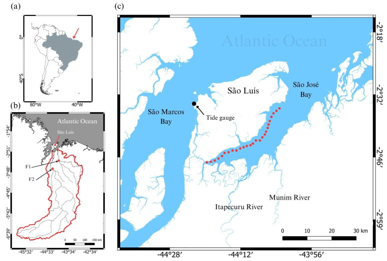
São José Bay (Figure 1) lies between São Luís Island from the mainland to the east. To the west, the island is separated by São Marcos Bay, and to the south, the Mosquito Strait interconnects the two bays (Ab’Sáber, 2001). This estuarine system is part of the Amazonian coast, which also encompasses the states of Pará and Amapá, and hosts one of the world’s largest continuous mangrove systems, covering approximately 8,900 km² (Kjerfve et al., 2002; Schettini et al., 2020). Of this total area, approximately 5,400 km² are located in Maranhão State (Kjerfve and Lacerda, 1993).

Figure 1
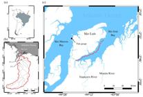
Location of the study area: (a) South America, (b) the drainage basin contributing to São José Bay, and (c) São José Bay, showing the data collection stations and the location of the tide gauge.

São José Bay extends approximately 63 km in length, with a maximum width of 15 km at its mouth, gradually narrowing upstream. The bay covers an area of approximately 580 km² (Furtado et al., 2025). Although no bathymetric charts are available, reports from local mariners and limited existing information indicate that the western portion of the bay features a deeper channel reaching depths of up to 20 m, while the eastern portion is shallower, with depths less than 5 m. The innermost regions also include extensive intertidal areas occupied by mangroves.

The local climate is transitional between the humid Amazonian climate and the semi-arid climate of northeastern Brazil, classified as an equatorial monsoon (Am) according to the Köppen-Geiger system. The climate is characterized by well-defined wet and dry seasons, controlled by the position of the Intertropical Convergence Zone (ITCZ). During the first half of the year, the ITCZ brings northeast trade winds that transport moist air masses and produce rainfall in the region (Ferreira et al., 2015). The average annual temperature in the city of São Luís is 26.8°C, with virtually no annual variation.

The Itapecuru and Munim Rivers are the main tributaries feeding into São José Bay, with drainage basins covering areas of 55,400 km² and 15,000 km², respectively (Figure 1). Together, they supply an average annual discharge of 164 m³/s, varying seasonally according to wet and dry regimes. The regional astronomical tide is purely semi-diurnal (Beardsley et al., 1995; Frota et al., 2016), with tidal heights ranging between 2.5 and 6 m during neap and spring tide conditions, respectively.

METHODS

Salinity distribution patterns in estuaries reflect the interactions between river discharge and tides within the estuarine basin. Accordingly, riverine contribution is first analyzed using secondary data, followed by an assessment of the tidal regime, also based on secondary data. Finally, the distribution of physical water properties is analyzed using oceanographic surveys conducted under different river discharge and tidal conditions.

FLUVIAL REGIME

The characterization of the river discharge regime involves assessing the temporal variability of freshwater input to the estuary to evaluate the buoyancy flux that may enhance stratification (Geyer and MacCready, 2014). Daily discharge data for the Itapecuru and Munim Rivers from 1963 to 2023 were used. These data were obtained from the Hidroweb database (https://www.snirh.gov.br/hidroweb/) maintained by the Brazilian National Water and Sanitation Agency (ANA). The fluviometric stations closest to the river mouths were selected. For the Itapecuru River, the “Cantanhede” station (#33680000) was chosen, with a drainage area of 51,129 km². For the Munim River, the “Nina Rodrigues” station (#33780000) was selected, with a drainage area of 12,600 km². These stations represent 96% and 79% of the total drainage areas of their respective basins.

Drainage basin delineation and area calculation was performed using vector files (shapefiles) of Brazil’s meso- and macro-basins, provided by the Brazilian Institute of Geography and Statistics (IBGE, 2023). These data were processed in QGIS software (https://qgis.org/), enabling calculation of total basin areas. Since drainage areas monitored by the fluviometric stations do not fully encompass the entire basins, river discharge was extrapolated proportionally to the total area. The manipulation and analysis of hydrological data were conducted using Python in a Jupyter environment (https://gutoschettini.github.io/IPYNB-Collection/17_Hidroweb_Flow_Climatology_PatosLagoon.html) (Schettini, 2021).

TIDAL REGIME

Tidal data were obtained from a tide gauge installed in the city of São José do Ribamar, located at 2°33’48” S/44°3’6” W (Figure 1). This tide gauge has been in continuous operation since 2018 and is maintained by the SIMCosta Project (www.simcosta.furg.br), with data transmitted via telemetry. Records are provided at a 15-minute sampling interval.

Harmonic analysis of the tides (Pugh, 1987) was performed using a 31-day dataset from October 2023. The analysis identifies the main harmonic constituents responsible for tidal variability and estimates their amplitudes and phases. The resulting constituents are then used to reconstruct the tidal time series for 2003, when hydrographic surveys were conducted in the bay (described below). The UTide package in Python was used for this analysis (https://pypi.org/project/UTide/), which is based on Codiga (2011). The tidal envelope, which represents the variation in tidal amplitude over time, was obtained by applying the Hilbert transform to the reconstructed tidal time series (https://gutoschettini.github.io/IPYNB-Collection/16_ComplexDemod_HilbertTrans.html) (Schettini, 2021).

ESTUARINE FLOW RATIO

The estuarine flow ratio (E _FR ) is a metric used to assess the relative importance of tides and river discharge in estuarine dynamics (Dyer, 1997). This parameter is defined as the ratio between the volume of fluvial water (V _f ) entering the estuary during half a tidal cycle and the volume of the tidal prism ((V _t ).

$E_{FR}=\frac{V_f}{V_t},$ (1)

where

$V_f={\int }_0^{6.2}Qdt,$ (2)

$V_t=h_{t}A,$ (3)

in which Q is the river discharge (m³/s), h _t is the tidal height (m), and A is the surface area of the estuary. River discharge was obtained from the time series of combined Itapecuru and Munim River discharges, extrapolated to the entire drainage basin for 2003. Tidal height, defined as twice the amplitude, was derived from the time series of the tidal envelope generated by the Hilbert Transform. The estuarine surface area was obtained using QGIS software by digitizing the bay’s coastline.

OCEANOGRAPHIC SURVEYS

Four oceanographic surveys were conducted to obtain salinity and temperature distributions, aiming to capture different tidal conditions (spring and neap tides) and hydrological regimes (dry and wet seasons) (Table 1). Sampling stations were distributed along a 40 km longitudinal transect, starting near the mouth at the village of São José do Ribamar, and proceeding upstream to the bay’s head at the entrance of the strait connecting both bays. Navigation was conducted along the western side of the bay, known by local mariners as the deepest portion. The number of stations varied for each survey, with an average spacing of approximately 2 km (Figure 1). Data were collected using a fast vessel, and the surveys were completed within roughly 2 hours, providing a quasi-synoptic snapshot of the property distributions. All navigation and georeferencing were performed using GPS.

Table 1
Surveys conducted to obtain the longitudinal distribution of physical properties along São José Bay, encompassing seasonal hydrological variation and synodic tidal regimes.

Date	Season	Tidal Phase	Start	End	Duration	Stations
18/Apr/2003	Wet	Spring	06:18	08:26	2:10	20
25/Apr/2003	Wet	Neap	10:15	11:36	1:19	19
17/Nov/2003	Dry	Neap	10:18	12:16	1:58	26
24/Nov/2003	Dry	Spring	15:04	17:12	2:08	25

At each station, navigation was halted and salinity and temperature profiles were collected using a SAIV A/S CTD profiler (https://saiv.no/sd204-ctd-profiler), operating at a sampling frequency of 1 Hz. According to the manufacturer, the instrument is equipped with long-term stability sensors, with a salinity resolution of 0.01±0.01 g/kg and a temperature resolution of 0.001±0.01 °C. The CTD was deployed vertically to the seabed at a controlled descent rate of 0.5 m/s. Data processing was performed using only the downcast measurements to minimize potential artifacts. The resulting profiles were linearly interpolated to a uniform vertical resolution of 0.5 m, consistent with the sampling frequency and descent rate. Subsequently, water density was computed from the CTD-derived salinity and temperature data using the seawater equation of state as implemented in the Seawater package for Python (https://pypi.org/project/seawater).

VERTICAL STRATIFICATION

The vertical structure of the water column, or degree of stratification, was assessed using three parameters: (1) the stratification parameter, (2) the buoyancy frequency, and (3) the potential energy anomaly (Frota et al., 2013). The stratification parameter is one of the dimensionless indices in the estuarine classification proposed by Hansen and Rattray Jr. (1966) and is originally calculated using salinity. In this study, density was used instead to enable comparison with other parameters. The stratification parameter, ε, is defined as:

$\epsilon =\frac{{\rho }_B-{\rho }_S}{\overline{\rho }},$ (4)

in which ρ_B is the bottom density, ρ_S is the surface density, and is the mean water column density. Values of ε range from 0, indicating fully homogeneous conditions, to 0.025, representing maximally stratified conditions.

The buoyancy frequency, N, also known as the Brunt-Väisälä frequency, quantifies the stability of the water column (Pond and Pickard, 1983), and is calculated as:

$N^2=\frac{-g}{{\rho }_O}\frac{\partial \rho }{\partial z}$ (5)

in which g is the acceleration due to gravity, ρ_O is a reference density, and z is the vertical coordinate, positive upward. In a stable water column, N represents the frequency at which a vertically displaced parcel oscillates around its isostatic level, depending on the potential energy gained relative to its resting position. Stronger stratification corresponds to higher N values. The highest values typically occur within the pycnocline, which, in coastal waters or estuaries, often coincides with the halocline (Pond and Pickard, 1983).

The potential energy anomaly, Φ, is another metric used to quantify stratification (Simpson and Sharples, 2012), and is defined as:

$\Phi =\frac{g}{h}{\int }_{-h}^0\left(\acute{\rho }-\rho \left(z\right)\right)zdz$ (6)

in which h is the depth of the water column. This parameter represents the energy required to fully mix the water column (J/m³). Under homogeneous conditions, equals zero. Its value increases with stratification, and typical values are on the order of tens. Variability in the potential energy anomaly reflects the energy balance over each tidal cycle: the greater the stratification, the more energy is required to homogenize the water column.

CLASSIFICATION OF THE ESTUARY

The system was classified following the framework proposed by Geyer and MacCready (2014). This approach uses a dimensional space defined by the freshwater Froude number and a mixing parameter. The former represents the role of river discharge in generating buoyancy-driven flow and stratification, while the latter quantifies the turbulence production induced by tidal forcing and the resulting vertical mixing.

The freshwater Froude number, which represents the velocity of river flow relative to the frontal propagation speed, is calculated as

$F{\gamma }_f=\frac{U_R}{{\left(\beta g{S}_{OC}h\right)}^{0.5}}$ (7)

in which U _R is the river flow velocity, obtained as the ratio of discharge to cross-sectional area, β is the halosteric contraction coefficient of seawater (7.7×10^-4), and S _OC is a reference value for coastal salinity (35 g/kg). The mixing parameter is defined as:

$M^2=\frac{C_D{U}_T^2}{\omega N_O{h}^2}$ (8)

in which C _D is the drag coefficient (0.0022), is the tidal current amplitude, ω is the M2 tidal angular frequency, and N _O is the buoyancy frequency corresponding to the maximum vertical salinity gradient in the estuary, given by N _O =(βgS _OC /H)^0.5.

Fγ_f , U _R was estimated using historical median values for the wet (~1,000 m3/s) and dry (~100 m3/s) seasons. A representative cross-sectional area for the bay was calculated using an average width of 8 km and mean depth of 15 m. The average width was determined by measuring the bay at 5 km intervals along its longitudinal axis using QGIS (https://qgis.org/). For the calculation of M, reference values for the tidal current amplitude (U _T ) were obtained from Acoustic Doppler Current Profiler (ADCP) deployments conducted during spring tide (November 23, 2003) and neap tide (November 16, 2003) conditions. A Nortek Aquadopp Profiler 1000 kHz ADCP recorded data at 30-minute intervals, covering a full semidiurnal tidal cycle (~13 hours).

CODE AVAILABILITY

Data processing and visualization were performed using the Python within the JupyterLab IDE. The processed datasets and main Jupyter notebooks (.ipynb files) are available in the GitHub repository: https://github.com/LuisOliveiraLago/Hydrodynamic_Characterization_SJB

RESULTS

FLUVIAL REGIME

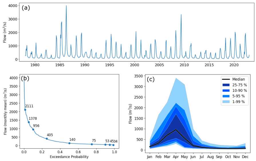
Figure 2a presents the historical time series of combined discharge from the Itapecuru and Munim rivers since 1978, highlighting the region’s seasonal hydrological variability. A clear distinction between the wet and dry seasons is observed, with peak discharges during rainy months and pronounced minima in the dry season. These consistent patterns over decades reflect the strong influence of the tropical climate regime on annual precipitation and river discharge. The median discharge was 140 m³/s, while the mean annual maximum was 1,300 m³/s, reaching minimum values around 35 m³/s (Figure 2b). The highest recorded discharges occurred in 1986 (3,220 m³/s) and 2009 (3,194 m³/s). Monthly discharge variability is greatest during the wet season and minimal during the dry season (Figure 2c). Peak discharges typically occur in April, with high-flow conditions extending from January to July, while the period from August to December is dominated by low flows.

Figure 2
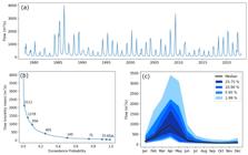
(a) Time series of the combined mean monthly discharge of the Itapecuru and Munim rivers since 1978; (b) Flow-duration curve showing discharge percentiles (1, 5, 10, 25, 50, 75, 90, 95, and 99); (c) Seasonal discharge climatology showing median variation and percentile ranges.

TIDAL REGIME

Figure 3 presents observed water level data for October 2023, underscoring a predominantly semidiurnal tidal pattern (12:40), followed by spring-neap variations. Spring tide heights reached up to 6 m, while neap tides reached approximately 2.5 m. Table 2 shows the amplitude and phase of the main harmonic constituents obtained from this time series. The tidal regime is dominated by the principal lunar semidiurnal constituent, with an amplitude exceeding 2 m, followed by the principal solar semidiurnal constituent, with an amplitude around 0.5 m. The dominance of the semidiurnal regime is confirmed by the tidal form number (F), defined as the ratio of the sum of diurnal constituent amplitudes (K₁+O₁) to the sum of semidiurnal constituent amplitudes (M₂+S₂), resulting in F=0.075. This value is well below the 0.25 threshold for semidiurnal tides (Pugh, 1987), indicating minimal diurnal inequalities between consecutive tides.

Figure 3
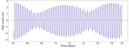
Water level variations during October 2023, showing the alternation between spring and neap tides, with maximum amplitudes during spring tides and minimum amplitudes during neap tides.

Table 2
Amplitude and phase values of the main tidal harmonic constituents determined by harmonic analysis for October 2023, at the tide gauge in Itaqui Port.

Component	Species	Amplitude (m)	Phase (degrees)
MSF	Lunisolar synodic fortnightly	0.045	8
O1	Lunar diurnal	0.107	216
K1	Lunisolar diurnal	0.098	238
M2	Principal lunar semidiurnal	2.167	196
S2	Principal solar semidiurnal	0.572	232
M4	Lunar quartidiurnal overtides	0.095	224

Tidal amplitudes varied considerably during October 2023. Spring tides, observed on the 6th and 21st, coincided with the full and new moon phases, exhibiting maximum amplitudes of up to 3.2 m. Neap tides, occurring on the 13th and 27th, showed reduced amplitudes, with average values of 1.4 m.

Tidal variations followed the lunar cycle, with approximately 14.8 days between consecutive spring tides. These results support the classification of the region as macrotidal, as maximum amplitudes exceed 2 m - a typical characteristic of tropical Atlantic coastal areas.

ESTUARINE FLOW RATIO

The flow ratio exhibited average values of 0.01 during the first half of 2003, corresponding to the rainy season, and 0.001 in the second half, corresponding to the dry season, representing an order-of-magnitude difference between these periods. During neap tides, the mean flow ratio was 0.01, approximately three times higher than during spring tides (0.003). On the survey days, the flow ratio varied from 0.009 (neap) to 0.011 (spring) during the rainy season, and from 0.0015 (neap) to 0.0006 (spring) during the dry season. All values remained below 0.03, indicating tidal dominance in the system’s dynamics throughout the year (Dyer, 1997), although river discharge contributes more significantly in the first half of the year.

OCEANOGRAPHIC CAMPAIGNS

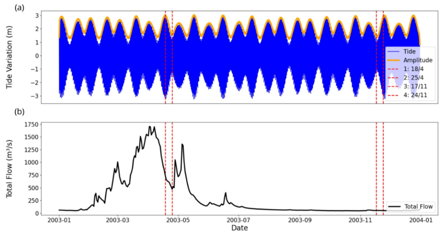
Tidal and river discharge conditions during the surveys are presented in Figure 4 regarding annual variations in tides and river flow. The tidal height during the neap tide survey in the rainy season was 2.7 m, with a river discharge of 940 m³/s. During the spring tide survey, the tidal height was 6.02 m, with a discharge of 631.9 m³/s. Tidal heights during the neap and spring tide surveys in the dry season were 2.42 m and 5.8 m, respectively, with corresponding discharges of 99 m³/s and 105 m³/s (Table 3).

Figure 4
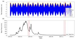
(a) Predicted water level variations for 2003, showing tidal amplitude fluctuations; (b) Combined daily discharge of the Itapecuru and Munim rivers in 2003. Red vertical lines indicate the dates of the oceanographic surveys.

Figure 5
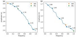
Exceedance probability curves for (a) spring and (b) neap tidal amplitudes, showing the 0.1, 0.25, 0.5, 0.75, and 0.9 percentiles. Orange and green circles indicate tidal amplitudes during the oceanographic surveys.

Figure 6
Time series of (a) total river discharge (Munim+Itapecuru), (b) tidal equivalent height derived from the Hilbert Transform, and (c) estuarine flow ratio throughout 2003 in the São José Bay.

Table 3
Tidal height, river flow, and mean salinity and temperature during each oceanographic campaign.

Campaign	Tidal height (m)	River flow (m3/s)	Salinity (g/kg)	Temperature (°C)
Wet/neap	2.8	940	1.5	29
Wet/spring	6.0	630	16	29
Dry/neap	2.4	99	31	29
Dry/spring	5.8	105	31.2	28.7

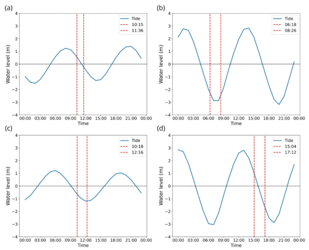
Figure 7 shows water level variations on the survey days, indicating the start and end of each campaign. All surveys were conducted within a relatively short timeframe compared to the tidal cycle. The rainy-season spring tide and dry-season neap tide campaigns were conducted during low tide, whereas the rainy-season neap tide and dry-season spring tide campaigns were conducted during ebb tide. Although the surveys did not coincide with the same tidal phase, the results remain representative for characterizing synodic conditions.

Figure 7
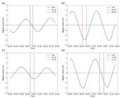
Water level variations for each day of the oceanographic surveys. Red vertical lines indicate the start and end of each survey.

Figure 5 shows the tidal amplitudes during each survey, demonstrating that the study successfully captured a wide range of tidal variation. Spring tide conditions exceeded the median amplitude, with the rainy-season campaign conducted under the maximum possible tidal amplitude. Similarly, both neap tide surveys were conducted under amplitudes below the median, with the dry-season campaign capturing the minimum neap amplitude.

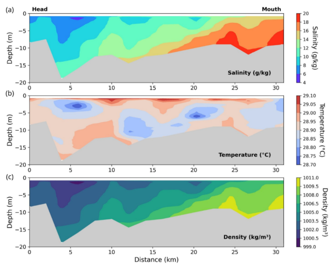
Figure 8 presents the longitudinal/vertical distributions of salinity, temperature, and density for the neap tide survey during the wet season. Salinity ranged from 4 to 20 g/kg, with the lowest values at the upstream surface, increasing towards the mouth. Seaward-tilted isohalines indicate stratification. Temperature ranged from 28.7 to 29.1 °C, with the highest values at the surface, showing no clear relationship with salinity distributions. Density closely followed the salinity distribution, ranging from 999 to 1,011 kg/m³.

Figure 8
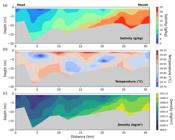
Longitudinal/vertical distribution of salinity (g/kg), temperature (°C), and density (kg/m³) along São José de Ribamar Bay during the wet season under neap tide conditions.

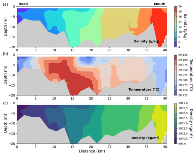
Figure 9 shows the longitudinal/vertical distributions of salinity, temperature, and density for the spring tide survey during the wet season. As the neap tide survey (Figure 8), salinity ranged from 4 to 20 g/kg, increasing from the head to the mouth, but with a less stratified vertical distribution compared to the neap tide survey. Water temperature also showed little variation, between 28.9 and 29.1 °C, with a notable patch of higher temperatures observed between 7 and 20 km and below the surface. Density closely followed the salinity variation, with values similar to those observed in the neap tide survey.

Figure 9
Longitudinal/vertical distribution of salinity (g/kg), temperature (°C), and density (kg/m³) along São José de Ribamar Bay during the wet season under spring tide conditions.

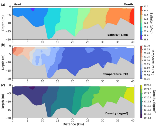
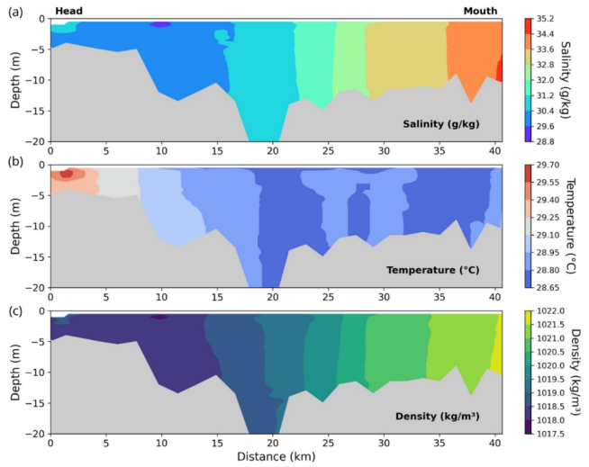
During the dry-season surveys, both during neap tide (Figure 10) and spring tide (Figure 11), salinity exhibited less variation (29-35 g/kg) compared to the wet season. However, a clear positive gradient from the head to the mouth persisted. In the neap tide survey, a slight tilt of the isohalines (stratification) is observable, whereas in the spring tide survey, vertical variation is virtually absent. Temperature exhibited considerably greater variability, between 28.3 and 29.7 °C, compared to the wet season surveys, in which variation was <0.5 °C. In both tidal conditions, a negative temperature gradient occurs from the head to the mouth. As observed during the wet season and in both tidal conditions, density during the dry season follows the salinity variation, with values ranging from 1,017 to 1,022 kg/m³.

Figure 10
Longitudinal/vertical distribution of salinity (g/kg), temperature (°C), and density (kg/m³) along São José de Ribamar Bay during the dry season under neap tide conditions.

Figure 11
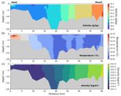
Longitudinal/vertical distribution of salinity (g/kg), temperature (°C), and density (kg/m³) along São José de Ribamar Bay during the dry season under spring tide conditions.

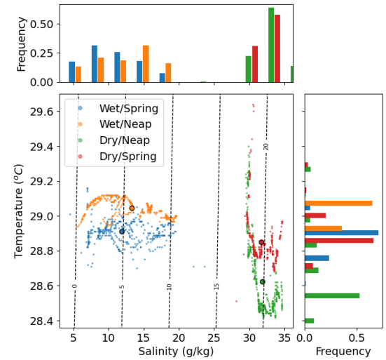
Figure 12 shows the temperature-salinity (TS) diagram for the four surveys, indicating mean salinity and temperature values for each campaign. Despite seasonal differences, the distribution patterns are relatively similar. Wet-season surveys present a smaller thermal range (δt~0.2 °C) but a larger salinity range (δs~15 g/kg). Conversely, dry-season surveys show a larger thermal range (δt~1 °C) and a smaller salinity range (δs~5 g/kg).

Figure 12
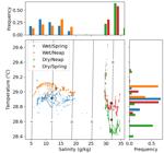
TS diagram showing hydrographic conditions observed during each campaign. Circles denote the center of gravity of all samples for each campaign. The panels on the top and left display the frequency histograms of temperature and salinity, respectively.

STRATIFICATION AND ESTUARINE CLASSIFICATION

Table 4 summarizes the estuarine flow ratio and stratification parameters for the four oceanographic surveys. Stratification parameters were generally higher during the wet season than in the dry season. Within each season, neap tide conditions produced higher stratification values than spring tides. However, during the wet season, the flow ratio was higher during the spring tide than the neap tide, reflecting the difference in river discharge between the surveys - around 900 m³/s during the spring tide and 600 m³/s during the neap tide.

Table 4
Estuarine flow ratio, stratification parameter, buoyancy frequency and potential energy anomaly during each oceanographic campaign.

Campaign	Flow Ratio (-)	Stratification Parameter (-)	Buoyancy Frequency (s-1)	Potential Energy Anomaly (J/m3)
Wet/neap	0.0032	0.0040	0.0031	24.21
Wet/spring	0.0042	0.0008	0.0011	4.07
Dry/neap	0.0005	0.0003	0.0003	2.72
Dry/spring	0.0002	0	0.0002	0.05

Based on the freshwater Froude number (Frf) and the mixing parameter (M), the classification of the Geyer and MacCready (2014) diagram is presented in Figure 13. Frf ranges from 0.001 in the dry season to 0.01 in the wet seasons, based on median historical values (Figure 2). The mixing parameter (M) ranged from 1.4 to 2.1, corresponding to observed tidal current amplitudes of 0.8 during neap tides and 1.2 m/s during spring tides. These values place the bay in a hydrodynamic regime of strain-induced periodic stratification (SIPS), similar to other bay environments, and are in good agreement with the findings of Santos et al. (2025) for São Marcos Bay.

Figure 13
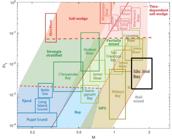
Estuarine parameter space based on the freshwater Froude number and the mixing number (Geyer and MacCready, 2014). The black rectangle indicates São José Bay, with vertical sides indicating synodic tidal variation and horizontal sides representing seasonal hydrological variability.

DISCUSSION

Salinity distribution and the degree of stratification are fundamental factors for understanding estuarine dynamics (Cloern et al., 2017). Both the longitudinal salinity distribution and stratification result from complex hydrodynamic interactions between buoyancy-driven flows from freshwater input and tidal currents, constrained by the estuarine basin (Dyer, 1997; Geyer, 2010; Geyer and MacCready, 2014; Miranda et al., 2002; Pritchard, 1955). Freshwater input follows a seasonal regime, typically on a half-year timescale (Charlton, 2007), while tidal currents vary hourly, with maximum intensity modulated by the synodic regime of spring and neap tides (Pugh, 1987).

Freshwater input to the bay follows the typical pattern of a humid tropical climate, with well-defined wet and dry seasons. Median monthly discharge during the wet season (1,000 m³/s) is an order of magnitude higher than during the dry season (100 m³/s). Wet-season discharge is historically regular but shows pronounced variability (Figure 2), associated with shifts in the ITCZ (Ferreira et al., 2015). In drought years, maximum discharge may drop below 300 m³/s, whereas in very wet years it may exceed 3,000 m³/s. Considering Maranhão State’s climatic transition between the Amazon and semi-arid northeastern Brazil, the hydrological regime suggests that estuarine dynamics are more similar to Amazonian estuaries (Asp et al., 2012, 2018) than to semi-arid estuaries, which may experience hypersaline conditions during the dry season (Schettini et al., 2017; Valle-Levinson and Schettini, 2016).

The tidal regime reflects the pattern of astronomical tides along the northern coast of Brazil, dominated by semidiurnal tides (Frota et al., 2016), with meso- to macro-tidal ranges (Beardsley et al., 1995) and minimal low-frequency, non-astronomical water level variations (e.g., Truccolo et al., 2006). Tidal ranges in São José Bay are considerably greater than in Fortaleza city, 700 km to the east. While diurnal harmonic constituents (K1 and O1) exhibit relatively similar values, the greater tidal range is mainly due to increases in M2 (from 106 to 216 cm) and S2 (from 34 to 57 cm). Although no direct tidal measurements exist within the bay, the tidal bore (“pororoca”) in the Mearim River at the head of São Marcos Bay (Kjerfve and Ferreira, 1993) suggests up-estuary tidal wave deformation and possible amplification. Despite the presence of intertidal flats at the head of the bay, the area is small compared to the total bay area, indicating that tidal deformation likely produces a flood-dominated system (Speer et al., 1991), with tidal pumping being key in material transport.

The oceanographic surveys successfully captured the full range of hydrological (wet and dry seasons) and synodic (spring and neap tides) variability. Ideally, the wet-season surveys could have been conducted slightly earlier, when discharge exceeded 1,500 m³/s. However, the baroclinic adjustment timescale for an estuary of São José Bay’s dimensions is relatively slow - on the order of weeks (MacCready, 1999). Longitudinal distributions of salinity and temperature along the bay were also reported by Santos et al. (2023) for 2017, covering both dry and wet seasons. Although these earlier surveys had lower spatial resolution and did not account for the tidal phase, the observed variation amplitudes are relatively consistent with the results of this study.

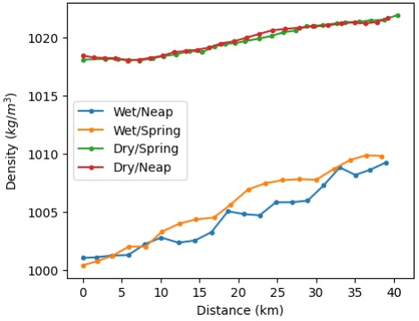
When expressed as percentages, the estuarine flow ration indicates that freshwater contributes approximately 1% of the tidal prism volume during the wet season, decreasing to about 0.1% in the dry season. These low values indicate a well-mixed estuary, in which freshwater input plays a secondary role (Dyer, 1997). Nevertheless, even with a significantly reduced freshwater contribution during the dry season, a dilution regime is maintained, with positive salinity and density gradients seaward (Figure 14), generating a baroclinic pressure gradient (BPG) (Geyer, 2010; Geyer and MacCready, 2014; Miranda et al., 2002). For reference, the BPG is given by:

$BPG=-\frac{g}{{\rho }_0}{\int }_z^{\eta }\frac{\partial \rho }{\partial x}dz$ (9)

Figure 14
Longitudinal variation of depth averaged density during the four oceanographic campaigns.

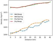
Considering density values at the head and mouth of the estuary and an average channel depth of 10 m, BPG values were approximately 2×10^-5 m/s² during the wet season and 9.6×10^-6 m/s² during the dry season. Differences between spring and neap tide conditions were minimal.

Temperature variability was less than 0.5 °C during the wet-season surveys and about 1 °C during the dry-season campaigns. Although temperature has a minor effect on water density, it is noteworthy that during the dry season, when solar radiation is higher, temperatures increase toward the estuarine head. This is likely due to shallower waters and extensive intertidal regions.

The bay exhibits the characteristics of a well-mixed estuary with a strain-induced periodic stratification (SIPS) regime, according to the framework proposed by Geyer and MacCready (2014). Stratification indices indicate that maximum stratification occurs during the wet season under neap tide conditions, positioning the system towards the upper-left corner of the parametric space for partially stratified systems. Functionally, during the dry season, the system behaves as well-mixed, with hydrodynamics primarily determined by tides. However, during the wet season, tides remain the principal driver of hydrodynamics, but freshwater-driven buoyancy flux becomes increasingly important, interacting with tidal forcing to generate periodic stratification during ebb flows (Simpson et al., 1990; Schettini et al., 2021).

The classification of São José de Ribamar Bay aligns closely with that of São Marcos Bay, according to the Geyer and MacCready (2014) framework, as reported by Santos et al. (2025). Both bays share similar morphology, climatic and tidal regimes, and drainage basin sizes, although São Marcos Bay is approximately twice as long with a larger surface area, reducing the relative influence of river discharge. The Pará River, located about 450 km to the west, is geomorphologically similar and subject to the same tidal regime. However, it receives inflow from the Tocantins and Amazon Rivers (Prestes et al., 2020), making it much larger. Consequently, while its hydrodynamics may resemble the Maranhão bays, the higher freshwater input likely produces more pronounced partially stratified conditions.

CONCLUSIONS

São José Bay, one of the largest estuaries in Brazil, drains a 70,000 km² tropical watershed with distinct wet (1,000 m³/s) and dry (100 m³/s) seasons. The semidiurnal tidal regime, dominated by the M2 constituent, produces ranges of 2.5 m under neap tide conditions to up to 6 m during spring tides.

Freshwater contributes only about 1% of the volume exchanged during tidal cycles in the wet season, decreasing to 0.1% in the dry season. The greater freshwater contribution during the wet season generates a buoyancy-driven flow that increases stratification. Consequently, the bay is well-mixed during the dry season and exhibits strain-induced periodic stratification during the wet season.

DATA AVAILABILITY STATEMENT

Data will be available under request.

SUPPLEMENTARY MATERIAL

There is no supplementary material for this article.

ACKNOWLEDGMENTS

We thank all those who contributed to the field surveys.

REFERENCES

• Ab’Sáber, A. N. 2001. Brazilian coast. São Paulo, Metalivros.
• Arruda-Santos, R. H. D., Schettini, C. A. F., Yogui, G. T., Maciel, D. C. & Zanardi-Lamardo, E. 2018. Sources and distribution of aromatic hydrocarbons in a tropical marine protected area estuary under influence of sugarcane cultivation. Science of The Total Environment, 624, 935-944. DOI: https://doi.org/10.1016/j.scitotenv.2017.12.174
  » https://doi.org/10.1016/j.scitotenv.2017.12.174
• Asp, N. E., Schettini, C. A. F., Siegle, E., Silva, M. S. & Brito, R. N. R., 2012. The dynamics of a fricctionlly-dominated Amazonian estuary. Brazilian Journal of Oceanography, 60(3), 391-403.
• Asp, N. E., Gomes, V. J. C., Schettini, C. A. F., Souza-Filho, P. W. M., Siegle, E., Ogston, A. S., Nittrouer, C. A., Silva, J. N. S., Nascimento, W. R., Souza, S. R., Pereira, L. C. C. & Queiroz, M. C. 2018. Sediment dynamics of a tropical tide-dominated estuary: turbidity maximum, mangroves and the role of the Amazon River sediment load. Estuarine, Coastal and Shelf Science, 214, 10-24. DOI: https://doi.org/10.1016/j.ecss.2018.09.004
  » https://doi.org/10.1016/j.ecss.2018.09.004
• Beardsley, R. C., Candela, J., Limeburner, R., Geyer, W. R., Lentz, S. J., Castro, B. M., Cacchione, D. & Carneiro, N. 1995. The M2 tide on the Amazon shelf. Journal of Geophysical Research, 100(C2), 2283-2319. DOI: https://doi.org/10.1029/94JC01688
  » https://doi.org/10.1029/94JC01688
• Burchard, H., Schuttelaars, H. M. & Ralston, D. K. 2018. Sediment trapping in estuaries. Annual Review of Marine Science, 10(1), 371-395. DOI: https://doi.org/10.1146/annurev-marine-010816-060535
  » https://doi.org/10.1146/annurev-marine-010816-060535
• Cameron, W. M. & Pritchard, D. W. 1963. Estuaries. In: Hill, M. N. (Ed.). The sea (pp. 700). New York: Wiley.
• Cloern, J. E., Jassby, A. D., Schraga, T. S., Nejad, E. & Martin, C. 2017. Ecosystem variability along the estuarine salinity gradient: examples from long-term study of San Francisco bay. Limnology and Oceanography, 62(S1), S272-S291. DOI: https://doi.org/10.1002/lno.10537
  » https://doi.org/10.1002/lno.10537
• Charlton, R. 2007. Fundamentals of fluvial geomorphology. London, Taylor and Francis.
• Codiga, D. L. 2011. Unified tidal analysis and prediction using the UTide Matlab functions (Technical Report 2011-01). Narragansett: Graduate School of Oceanography, University of Rhode Island.
• Dyer, K. R. 1995. Chapter 14 Sediment Transport Processes in estuaries. Developments in Sedimentology, 53, 423-449. DOI: https://doi.org/10.1016/S0070-4571(05)80034-2
  » https://doi.org/10.1016/S0070-4571(05)80034-2
• Dyer, K. R. 1997. Estuaries: A Physical Introduction. New York: John Willey and Sons.
• Fairbridge, R. W. 1980. The Estuary: its Definition and geodynamic cycle. Chemistry and Biochemistry of Estuaries, 1-36.
• Ferreira, D. B. S., Souza, E. B., Moraes, B. C. & Meira Filho, L. G., 2015. Spatial and temporal variability of rainfall in eastern Amazon during the rainy season. The Scientific World Journal, 2015(1), 209783. DOI: http://dx.doi.org/10.1155/2015/209783
  » http://dx.doi.org/10.1155/2015/209783
• Freitas, P. P., Menezes, M. O. B. & Schettini, C. A. F. 2015. Hydrodynamics and particulate suspended matter transport in a shallow and highly urbanized estuary: the Cocó estuary, Fortaleza, Brazil. Brazilian Journal of Geophysics, 33(4), 1-12. DOI: https://doi.org/10.22564/rbgf.v33i4.754
  » https://doi.org/10.22564/rbgf.v33i4.754
• Frota, F. F., Paiva, B. P. & Schettini, C. A. F. 2013. Intra-Tidal variation of stratification in a semi-arid estuary under the impact of flow regulation. Brazilian Journal of Oceanography, 61(1), 23-33. DOI: https://doi.org/10.1590/S1679-87592013000100003
  » https://doi.org/10.1590/S1679-87592013000100003
• Frota, F. F., Truccolo, E. C. & Schettini, C. A. F., 2016. Tidal and sub-tidal sea level variability at the northern shelf of the Brazilian Northeast Region. Anais da Academia Brasileira de Ciências, 88(3), 1371-1386.
• Furtado, J. A., Cavalcanti-Lima, L. F., Santos, V. H. M., Serejo, J. H. F., Pereira, L. C. C., Carvalho-Neta, R. N. F. & Tchaicka, L. 2025. Multimetric trophic status and harmful algal species in a harbor area of the Amazon macrotidal mangrove coast. Ecohydrology & Hydrobiology, 25(3), 618-631. DOI: https://doi.org/10.1016/j.ecohyd.2024.10.002
  » https://doi.org/10.1016/j.ecohyd.2024.10.002
• Geyer, W. R. 2010. Estuarine salinity structure and circulation. In: Valle-Levinson, A. (Ed.) Contemporary Issues in Estuarine Physics (pp. 11-26). Cambridge, Cambridge University Press.
• Geyer, W. R. & MacCready, P. 2014. The estuarine circulation. Annual Review of Fluid Mechanics, 46, 175-197. DOI: https://doi.org/10.1146/annurev-fluid-010313-141302
  » https://doi.org/10.1146/annurev-fluid-010313-141302
• Hansen, D.V. & Rattray Jr., M. 1966. New Dimensions in estuary classification. Limnology and Oceanography, 11(3), 319-326. DOI: https://doi.org/10.4319/lo.1966.11.3.0319
  » https://doi.org/10.4319/lo.1966.11.3.0319
• Jago, C., Robins, P., Howlett, E., Hassard, F., Rajko-Nenow, P., Jackson, S., Chien, N. & Malham, S. 2024. Trapping and bypassing of suspended particulate matter, particulate nutrients and faecal indicator organisms in the river-estuary transition zone of a shallow macrotidal estuary. Science of The Total Environment, 917, 170343. DOI: https://doi.org/10.1016/j.scitotenv.2024.170343
  » https://doi.org/10.1016/j.scitotenv.2024.170343
• Kjerfve, B. & Ferreira, H. O. 1993. Tidal bores: first ever measurements. Ciência e Cultura, 45(2): 135-138.
• Kjerfve, B. & Lacerda, L. D. 1993. Conservation and sustainable utilization of mangrove forest in Latin America and Africa regions. In: Lacerda, L. D. (ed.). Mangroves of Brazil. International Society for Mangrove Ecosystems, Okinawa, 245-272.
• Kjerfve, B., Perillo, G. M. E., Gardner, L. R., Rine, J. M., Dias, G. T. M. & Mochel, F. R. 2002. Chapter twenty morphodynamics of muddy environments along the Atlantic coasts of North and South America. Proceedings in Marine Science, 4, 479-532. DOI: https://doi.org/10.1016/S1568-2692(02)80094-8
  » https://doi.org/10.1016/S1568-2692(02)80094-8
• Lima, H. P., Dias, F. J. S., Teixeira, C. E. P., Godoi, V. A., Torres, A. R. & Araújo, R. S., 2021. Implications of turbulence in a macrotidal estuary in Northeastern Brazil: The São Marcos estuarine complex. Regional Studies in Marine Science, 47, 101947. DOI: https://doi.org/10.1016/j.rsma.2021.101947
  » https://doi.org/10.1016/j.rsma.2021.101947
• Levin, L. A., Boesch, D. F., Covich, A., Dahm, C., Erséus, C., Ewel, K. C., Kneib, R. T., Moldenke, A., Palmer, M. A., Snelgrove, P., Strayer, D. & Weslawski, J. M. 2001. The function of marine critical transition zones and the importance of sediment biodiversity. Ecosystems, 4(5), 430-451. DOI: https://doi.org/10.1007/s10021-001-0021-4
  » https://doi.org/10.1007/s10021-001-0021-4
• MacCready, P. 1999. Estuarine adjustment to changes in river flow and tidal mixing. Journal of Physical Oceanography, 29(4), 708-726.
• Miranda, L. B., Castro, B. M. & Kjerfve, B. 2002. Princípios de Oceanografia Física de estuários. São Paulo, EdUSP.
• Pond, S. & Pickard, G. L. 1983. Introductory Dynamical Oceanography. New York, Pergamon Press.
• Prestes, Y. O., Borba, T. A. C., Silva, A.C. & Rollnic, M. 2020. A Discharge stationary model for the Pará-Amazon estuarine system. Journal of Hydrology: Regional Studies, 28, 100668. DOI: https://doi.org/10.1016/j.ejrh.2020.100668
  » https://doi.org/10.1016/j.ejrh.2020.100668
• Pritchard, D. W. 1955. Estuarine circulation patterns. Proceedings of the American Society of Civil Engineers, 81(717), 1-11.
• Pugh, D. T. 1987. Tides, surges and mean sea level: a handbook for engineers and scientists. Chichester, John Wiley & Sons.
• Santos, V. H. M., Dias, F. J. S., Torres, A. R., Soares, R. A., Terto, L. C., Castro, A. C. L., Santos, R. L. & Cutrim, M. V. J. 2020. Hydrodynamics and suspended particulate matter retention in macrotidal estuaries located in Amazonia-Semiarid interface (Northeastern Brazil). International Journal of Sediment Research, 35(4), 417-429. DOI: https://doi.org/10.1016/j.ijsrc.2020.03.004
  » https://doi.org/10.1016/j.ijsrc.2020.03.004
• Santos, V. H. M., Dias, F. J. S., Dottori, M., Torres Júnior, A. R., Santos, R. L., Soares, O. A., Ribeiro Júnior, J. C. M., Serejo, J. H. F., Lima, H. P. & Azevedo, I. H. R. 2023. Investigation of Physical properties and suspended matter discharge in a macrotidal estuary at the Amazon-Semiarid transition zone. Regional Studies in Marine Science, 67, 103194. DOI: https://doi.org/10.1016/j.rsma.2023.103194
  » https://doi.org/10.1016/j.rsma.2023.103194
• Santos, V. H. M., Dias, F. J. S., Torres Júnior, A. R., Sousa-Filho, P. W. M., 2025. Estuarine circulation in a tropical macrotidal estuary on the Amazon coast: Relating thermohaline structure and suspended particulate matter concentrations. Estuaries and Coasts, 48(121), 121. DOI: https://doi.org/10.1007/s12237-025-01562-9
  » https://doi.org/10.1007/s12237-025-01562-9
• Schettini, C. A. F. 2021. Ocean data analysis with Python/Jupyter. Available from: Available from: https://gutoschettini.github.io/Ocean-Data-Analysis-Python/ Accessed date: 2024 April.
  » https://gutoschettini.github.io/Ocean-Data-Analysis-Python/
• Schettini, C.A.F. & Toldo Jr., E. E. 2006. Fine sediment transport modes in the Itajaí-Açu estuary, Southern Brazil. Journal of Coastal Research, (39), 515-519.
• Schettini, C. A. F., Pereira, M. D., Siegle, E., Miranda, L. B. & Silva, M. P. 2013. Residual fluxes of suspended sediment in a tidally dominated tropical estuary. Continental Shelf Research, 70, 27-35. DOI: https://doi.org/10.1016/j.csr.2013.03.006
  » https://doi.org/10.1016/j.csr.2013.03.006
• Schettini, C. A. F., Valle-Levinson, A. & Truccolo, E. C. 2017. Circulation and transport in short, low-inflow estuaries under anthropogenic stresses. Regional Studies in Marine Science, 10, 52-64. DOI: https://doi.org/10.1016/j.rsma.2017.01.004
  » https://doi.org/10.1016/j.rsma.2017.01.004
• Schettini, C. A. F., Asp, N. E., Ogston, A. S., Gomes, V. J. C., McLachlan, R. L., Fernandes, M. E. B., Nittrouer, C. A., Truccolo, E. C., & Gardunho, D. C. L., 2020. Circulation and fine-sediment dynamics in the Amazon macrotidal mangrove coast. Earth Surface Processes and Landforms, 45(3), 574-589. DOI: https://doi.org/10.1002/esp.4756
  » https://doi.org/10.1002/esp.4756
• Schettini, C. A. F., Silva, L. A., Valença, L. M. M. & Manso, V. A. V. 2021. Transport Processes in the Santa Cruz Channel, Brazil. Regional Studies in Marine Science, 45, 101812. DOI: https://doi.org/10.1016/j.rsma.2021.101812
  » https://doi.org/10.1016/j.rsma.2021.101812
• Schubel, J. R. & Carter, H. H. 1984. The estuary as a filter for fine-grained suspended sediment. In: Kennedy, V. S. (ed.). The estuary as a filter for fine-grained suspend ed sediment. The Estuary as a Filter, 81-105. DOI: https://doi.org/10.1016/B978-0-12-405070-9.50011-6
  » https://doi.org/10.1016/B978-0-12-405070-9.50011-6
• Simpson, J. H., Brown, J., Matthews, J. & Allen, G. 1990. Tidal straining, density currents, and stirring in the control of estuarine stratification. Estuaries and Coasts, 13, 125-132.
• Simpson, J. H., Sharples, J. 2012. Introduction to the physical and biological oceanography of shelf seas. Cambridge, Cambridge Univeristy Press.
• Speer, P. E., Aubrey, D. G. & Friedrichs, C. T. 1991. Nonlinear hydrodynamics of shallow tidal inlet/bay systems. In: Parker, B. B. (Ed.), Tidal hydrodynamics (pp. 321-339). New York: John Wiley & Sons.
• Truccolo, E. C., Franco, D. & Schettini, C. A. F. 2006. The low frequency sea level oscillations in the northern coast of Santa Catarina, Brazil. Journal of Coastal Research, 39(SI), 547-552.
• Valle-Levinson, A. & Schettini, C. A. F. 2016. Fortnightly switching of residual flow drivers in a tropical semiarid estuary. Estuarine, Coastal and Shelf Science, 169, 46-55. DOI: https://doi.org/10.1016/j.ecss.2015.12.008
  » https://doi.org/10.1016/j.ecss.2015.12.008
• Wolanski, E. & Ridd, P. 1986. Tidal mixing and trapping in mangrove swamps. Estuarine, Coastal and Shelf Science, 23(6), 759-771. DOI: https://doi.org/10.1016/0272-7714(86)90073-9
  » https://doi.org/10.1016/0272-7714(86)90073-9

• AI USE STATEMENT
  Generative ai tools, such as chatgpt, were used for language editing and improving the clarity of the manuscript. All intellectual content, research design, and data analysis were conducted solely by the authors.
• FUNDING
  Luis Lago acknowledges the Brazilian National Science Council (CNPq) for his scholarship. Carlos Schettini acknowledges support from CNPq (Grant #316037/2021-4).

Edited by

• Associate Editor:
  Eduardo Siegle

Publication Dates

• Publication in this collection
  09 Mar 2026
• Date of issue
  2026

History

• Received
  25 May 2025
• Accepted
  27 Nov 2025