FASTER MIXED-INTEGER QUADRATIC CONIC PROGRAMS FOR TWO COMPETITIVE MULTIPLE ALLOCATION P-HUB LOCATION PROBLEMS

ABSTRACT

We present new mixed-integer quadratic conic formulations for two variants of the multiple-allocation p-hub location problems in a competitive environment. The problems consist in locating p hubs so that an entrant company can establish its hub-and-spoke network to provide transportation services for pairs of origin-destination that exchange flows in a competitive market. The objective is to maximize the entrant’s market share when compared to its competitors. Both problems assume that the paths used to route the flows have one or at most two hubs. However, whereas the first problem allows an origin-destination to be serviced by multiple routes, the second problem requires that a single path be used. Here, we show that instead of maximizing the entrant’s market share, it is computationally more interesting to minimize the market lost so that equivalent, but more suitable programs to conic solvers can be obtained. When solved by a commercial conic programming solver, our proposed formulations achieve average speedups of 89 times for the multi-path variant and 37 times for the single-path variant, as shown in our extensive computational experiments on solving well-known datasets. Therefore, this work not only reformulates the problem but also substantially outperforms all prior works, demonstrating the practical applicability and effectiveness of our approaches.

Keywords:
hub location; competitive facility location; mixed-integer quadratic conic programming; mixed-integer non-linear optimization

1 INTRODUCTION

We address two variants of the multiple-allocation p-hub location problem (O’Kelly, 1986, 1987) in a competitive market. Generally speaking, the problems consist of locating p hub facilities to design a hub-and-spoke network for an entrant company that wishes to offer transportation services in a competitive market where pairs of origin-destination points that exchange flows can choose the services of different providers. This problem encapsulates a strategic decision-making process, where the objective is not merely to optimize network efficiency, but to do so in a competitive environment, in which customer choice is influenced by factors such as price, travel time, and service attractiveness. Such scenarios are common-place in industries such as air transportation, freight logistics, and telecommunications, where the design of an efficient hub-and-spoke network becomes a decisive factor for competitiveness and market share acquisition.

Hubs are facilities responsible for consolidating flows from different origins before routing them either to their final destinations or to another hub that will then distribute these flows to their final destinations. Bundling flows in interhub connections allows the entrant company to realize scale economies, which can lead to lower transportation costs than directly connecting the origin-destination points (O’Kelly, 1986; O’Kelly & Bryan, 1998). Traditionally, it is assumed that any path connecting a pair of origin-destination points has one or at most two hubs, although there are other variants of hub location problems that completely disregard this assumption (Contreras & O’Kelly, 2019).

Here, different companies compete non-cooperatively for the market by offering transportation services with varying relative utilities, e.g., price, travel time, service and transportation convenience, or company attractiveness. Customers usually choose the most appealing transportation service based on these relative utilities (Huff, 1964, 1966). The entrant company must then take these characteristics into account during the design of its hub-and-spoke network if it wants to maximize the captured market share (Eiselt & Marianov, 2009; Tiwari et al., 2021a,b). Note that, generally, companies focus on their individual gains, which are greatly affected by the location of their hubs. The success of an entrant company in capturing a larger market share is substantially influenced by the attractiveness of its hubs and their ability to sway customer behavior (Drezner & Drezner, 2001).

In the literature, this problem has been modeled with two different assumptions regarding how origin-destination points are connected to the hub network. Eiselt & Marianov (2009) and Tiwari et al. (2021a) have assumed that every pair of origin-destination points can interact with every installed hub of the network, thus allowing a multitude of paths to serve any pair of origin-destination points. We have dubbed this problem the multi-path multiple allocation p-hub location problem (MPMAPHLP). Tiwari et al. (2021b) have criticized this assumption, arguing that it prevents the aggregation of flows at the installed hubs and, therefore, hinders the exploitation of scale economies in inter-hub connections.

Tiwari et al. (2021b) have then proposed the assumption that only a single path should be used to route the flows of a given pair of origin-destination points to make it resemble the traditional multiple allocation variants of the hub location literature (Campbell & O’Kelly, 2012). We have named this variant the single path multiple allocation p-hub location problem (SPMAPHLP). Regardless of the adopted assumption, the problem gives rise to a difficult mixed-integer non-linear program that challenges existing off-the-shelf solvers. Thus, to solve such a problem, one needs to rely on different solution strategies.

For the problem involving the MPMAPHLP, Eiselt & Marianov (2009) have proposed a multi-start two-phase metaheuristic. In the first phase, for a given number of iterations, a random solution is generated and then improved by means of a local search that swaps an installed hub for a closed one. Whenever an improved solution is found, it is saved in a fixed-size list containing the overall best solutions from all iterations. The hubs of the solutions in this list form a concentration set that is used in the second phase of their algorithm. Again, for a given number of iterations, p hubs are randomly selected from the concentration set to form a solution to be improved using a local search procedure that now swaps two installed hubs for two closed ones belonging to the concentration set. The overall best solution is saved and returned at the end of the method.

For their turn, Tiwari et al. (2021a) have proposed four different approaches to solve the MPMAPHLP. Tiwari et al. have devised a Kelley cutting-plane algorithm, a reformulation based on a mixed-integer quadratic conic program (MIQCP), and Lagrangian relaxation-based algorithms using their first two methods as solvers for the Lagrangian subproblems. Tiwari et al. have made the source code for their implementation of their methods available online. Unfortunately, during the coding of their methods, Tiwari et al. typed the variable representing the scale economies in the inter-hub connections as an integer instead of setting it to float or double, thereby rendering their results biased or less insightful. For a given instance, the induced hub-and-spoke network was the same for the different tested values for the scale economy, as reported in their computational experiment tables, preventing a proper analysis of their reported results.

Tiwari et al. (2021b) have also proposed the same four previous solution strategies to address the SPMAPHLP. Once again, Tiwari et al. have typed their variable to represent the scale economy in their computer source code as an integer variable instead of a float or double, thus leading to biased or questionable results. Moreover, though they have assumed that only one path is used to route the flows for a given pair of origin-destination points, thus requiring a binary variable to represent whether a path is used or not, Tiwari et al. have relaxed this requirement by setting these variables to be non-negative within zero and one, which allowed their procedures to return dual bounds for the problem.

In their computational experiments, Tiwari et al. (2021a,b) have shown that their MIQCPs were competitive compared to their other devised approaches for solving instances with different arrangements for the number of hubs and scale economies in the Civil Aeronautics Board (CAB) dataset, using CPLEX as their conic solver set to run for one or two hours, respectively. Their MIQCPs have proven to be interesting tools for designing hub-and-spoke networks.

Here, we show a better way to reformulate both the MPMAPHLP and SPMAPHLP problems to obtain equivalent ones, but with the objective function of minimizing the market loss instead of maximizing the captured market share. This simple yet crucial approach leads to more lean and mean MIQCPs that have attained speed-ups of 89 and 37 times on average for the MPMAPHLP and SPMAPHLP problems, respectively, substantially outperforming the MIQCPs of Tiwari et al. (2021a,b) when solving the same set of computational experiments.

The remainder of this work is organized as follows. Section 2 presents the adopted notation and definitions and formally describes both problems. Section 3 underscores the differences between the proposed MIQCPs and those in the literature; while Section 4 discusses the attained numerical experiments. Finally, Section 5 concludes with our final remarks and suggestions for future work.

2 NOTATION, DEFINITIONS AND FORMULATIONS

Both MPMAPHLP and SPMAPHLP problems use the same underlying notation and definitions. Let N be the set of points scattered in a geographic region, in which each point i ∈ N is both a hub candidate and an origin or a destination for some demands. Let $W=\left\{\right(i,j)\in N\times N:i\ne j\}$ be the set of pairs of origin-destination points , with each pair (i, j) ∈ W exchanging w _ij > 0 units of flow. Let $I=\left\{\right(k,l)\in N\times N\}$ also be the set of all possible interhub connections or hub-pairs. There is also a set C of competitors that are already operating with a hub-and-spoke structure and competing for their respective market share, and an entrant company e that wishes to enter this market.

Although demand information is common knowledge for all competitors, no other information or infrastructure is shared between them; i.e., the companies do not cooperate. Moreover, each company a ∈ C ∪ {e} must operate its own sets H ^a ⊂ N and $I^a=\left\{\right(k,l)\in H^a\times H^a\}$ of installed hubs and active interhub connections, respectively, that may be used to form paths to route the captured demands. Recall that each path has one or two hubs, and that whenever two different hubs are used to transport the bundle of demand flows, scale economies can be exploited. Here, scale economies are represented by the scalar parameter α ∈ [0, 1].

Any entrant company seeks to capture the maximum market share possible by installing p hubs to form paths that can attract most of the demand from the origin-destination points (i, j) ∈ W . Note that each path i − k − l − j, with (i, j) ∈ W and (k, l) ∈ I ^a , operated by a company a ∈ C ∪ {e}, has a perceived utility $u_{iklj}^a$ can be written as for the demand w _ij , which follows a probabilistic choice model that can be written as

$u_{iklj}^a=\frac{A_{kl}^a}{\gamma (T_{iklj}^a{)}^{\beta }+(1-\gamma \left)\right(B_{iklj}^a{)}^{\delta }}.$

$A_{kl}^a$ represents the attractiveness of the interhub connection (k, l) ∈ I ^a and its respective hubs, while $B_{iklj}^a$ and $T_{iklj}^a$ are the cost and travel time, respectively, of the path. Parameters β and δ are scalar values that estimate the impact of travel time and cost, respectively, on the selection behavior of the demands. Higher power values indicate a dislike for longer travel times or higher transportation costs. Parameter γ represents the weight of the relative importance of each factor (cost and time) in the utility of the path. Moreover, parameters $B_{iklj}^a$ and $T_{iklj}^a$ are equal to c _ik + αc _kl + c _lj and t _ik +t _kl +t _lj , respectively, for all (i, j) ∈ W , (k, l) ∈ I, and a ∈ C ∪{e}, where c _ij and t _ij , i, j ∈ N are the unitary transportation cost and the travel time between points i, j, respectively.

The utility parameters are then used in an attraction function $f_{ij}^e$ that returns the amount of demand w _ij for the origin-destination pair (i, j) ∈ W that the entrant company e will capture with its available paths formed by its set I ^e of hub-pairs or interhub connections or:

$f_{ij}^e=w_{ij}\frac{{\displaystyle \sum _{(k,l)\in I^e}{u}_{iklj}^e}}{{\displaystyle \sum _{a\in C\cup \left\{e\right\}}\sum _{(k,l)\in I^a}{u}_{iklj}^a}}=w_{ij}\frac{{\displaystyle \sum _{(k,l)\in I^e}{u}_{iklj}^e}}{{\displaystyle \sum _{(k,l)\in I^e}{u}_{iklj}^e+{\mathcal{U}}_{ij}^c}}$

in which ${\mathcal{U}}_{ij}^c=\sum _{a\in C}\sum _{(k,l)\in I^a}{u}_{iklj}^a$ is introduced to simplify notation hereafter.

Note that while sets H ^a and I ^a are known for competitors a ∈ C, sets H ^e and I ^e that maximize the total captured demand must be found for the entrant company e. Note also that the cardinality of set H ^e is equal to p, since exactly p hubs will be installed for the entrant company e. Furthermore, to find these sets or the underlined configuration of hubs and active interhub connections, function $f_{ij}^e$ needs to be properly adjusted to comply with the respective assumptions of the MPMAPHLP and SAMAPHLP problems, which, given the nature of the function $f_{ij}^e$, are initially modeled as mixed-integer non-linear programs (MINLP). Table 1 summarizes the main notation. However, additional definitions for auxiliary parameters and decision variables might be required when recasting the current mixed-integer nonlinear programs into conic programs in Section 3.

Table 1
Summary of the main notation.

	Main notation
N	Set of points. |N| = n.
W	Set of origin destination pairs.
I	Set of all possible interhub connections.
α	Economy-of-scale factor for interhub connections.
$A_{kl}^a$	Attractiveness of the interhub connection (k, l) ∈ I a .
$B_{iklj}^a$	Cost of path i-k-l-j.
$T_{iklj}^a$	Travel time of path i-k-l-j.
β	Travel time impact estimator for the probabilistic choice model.
δ	Travel cost impact estimator for the probabilistic choice model.
γ	Weights between travel costs and travel times in the probabilistic choice model.
$f_{ij}^e$	The attraction function for market capture.
fij (w)	The captured market as a function of ω.
ϕij (w)	The market loss as a function of ω.
C	Set of competitors.
e	Entrant company.
I	$I=\left\{\right(k,l)\in N\times N\}$ or set of hub-pairs or interhub connections.
H a	Set of operating hubs of company a ∈ C ∪ {e}.
I a	Set of operating hub-pairs or interhub connections of company a ∈ C ∪ {e}.
W	$W=\left\{\right(i,j)\in N\times N:i\ne j\}$ or set of demand pairs of origin-destination points that exchange flows.
w ij	Demand of origin-destination pair (i, j) ∈ W.
p	Number of hubs to install.
$u_{iklj}^a$	The utility or attractiveness of path (i, k, l, j) of company a ∈ C ∪ {e}, (i, j) ∈ W and (k, l) ∈ I a .
${\mathcal{U}}_{ij}^c$	${\mathcal{U}}_{ij}^c=\sum _{a\in C}\sum _{(k,l)\in I^a}{u}_{iklj}^a$ is the competitions’ total attractiveness for the pair of origin-destination points (i, j) ∈ W.
πiklj	$\frac{u_{iklj}^e}{{\mathcal{U}}_{ij}^c}$, (i, j) ∈ W , (k, l) ∈ I.
yk ∈ {0, 1}	Decides the installation of hub k.
ωkl ∈ {0, 1}	Decides the installation of interhub connection (k, l).
xikl j ∈ {0, 1}	Decides the adoption of path i-k-l-j.
Qij ≥ 0, (i, j) ∈ W	Auxiliary variables required for the conic reformulations.
Vij ≥ 0, (i, j) ∈ W	Auxiliary variables required for the conic reformulations.
rij ≥ 0, (i, j) ∈ W	Auxiliary variables required for the conic reformulations.

2.1 The maximization form for the MPMAPHLP problem

In the MPMAPHLP problem, an entrant company e wants to enter a market for the transportation of flows between pairs of origin-destination points that seek the most attractive service among competing companies. The entrant company e plans to maximize its captured market share by installing p hubs to form its hub-and-spoke network. It is assumed that each competitor can use multiple paths that go through different hubs or hub-pairs to serve any pair of points (i, j) ∈ W.

To formulate the MPMAPHLP, Eiselt & Marianov (2009) have defined the decision variables of location y _k ∈ {0, 1}, which assume a value of one if a hub is installed at a point k ∈ N, and zero otherwise; and the activation of hub-pairs or interhub connections ω _kl ∈ {0, 1}, which assume a value of one if the interhub connection or hub-pair (k, l) ∈ I is set, and zero otherwise. Note that the decision variables ω _kl assemble the set I ^e of the entrant company. With the aid of these decision variables, Eiselt & Marianov have adjusted the attraction function for the pair of origin-destination points (i, j) ∈ W as

$f_{ij}\left(\omega \right)=w_{ij}\frac{{\displaystyle \sum _{(k,l)\in I}{u}_{iklj}^e{\omega }_{kl}}}{{\displaystyle \sum _{(k,l)\in I}{u}_{iklj}^e{\omega }_{kl}+{\mathcal{U}}_{ij}^c}}$

and then modeled the problem as follows:

$\mathbf{\text{MAXMPMAPHLP}}\left\{\begin{array}{l}\max \sum _{(i,j)\in W}{w}_{ij}\frac{{\displaystyle \sum _{(k,l)\in I}{u}_{iklj}^e{\omega }_{kl}}}{{\displaystyle \sum _{(k,l)\in I}{u}_{iklj}^e{\omega }_{kl}+{\mathcal{U}}_{ij}^c}}\left(1\right)\\ \text{s.t.:}{\omega }_{kl}\le y_k\forall (k,l)\in I\left(2\right)\\ {\omega }_{kl}\le y_l\forall (k,l)\in I\left(3\right)\\ \mathbf{}\mathbf{}\mathbf{}\sum _{k\in N}{y}_k=p\left(4\right)\\ y_k\in \{0,1\}\forall k\in N\left(5\right)\\ {\omega }_{kl}\in \{0,1\}\forall (k,l)\in I\left(6\right)\end{array}\right.$

The objective function (1) maximizes the captured demand of the entrant company. Constraints (2) and (3) are the activation constraints. The hub-pair or interhub connection (k, l) ∈ I can only be active if the respective hubs are installed. Constraint (4) guarantees that p hubs will be installed. The domain of the decision variables are shown in constraints (5) and (6).

Note that the MAXMPMAPHLP formulation is an integer nonlinear program (INLP) that can be transformed into a mixed-integer nonlinear program (MINLP) by relaxing the decision variables ω _kl ∈ [0, 1], (k, l) ∈ I. As the attractiveness function is a concave, smooth, and differentiable function, and since we wish to maximize the captured market share, whenever both y _k and y _l assume the value of one, then w _kl will also assume the value of one. See constraints (2) and (3). Nevertheless, whenever either y _k or y _l is equal to zero, w _kl assumes the value of zero. Hence, we shall replace constraints (6) hereafter with their relaxations.

2.2 The maximization form for the SPMAPHLP problem

The formulation MAXMPMAPHLP for the MPMAPHLP problem assumes that every point is connected to every hub, thereby enabling a large number of paths to serve any pair of origin-destination points that exchange flows. Tiwari et al. (2021b) have then proposed a variant that restricts the number of paths to a single one, giving rise to the single-path multiple allocation p-hub location (SPMAPHLP). Tiwari et al. have then adapted the attractiveness function using decision variables x _iklj ∈ {0, 1} that assume the value of one if the path (i, k, l, j), (i, j) ∈ W and (k, l) ∈ I, is used to route the flow demand w _ij and zero otherwise. The attractiveness function is written as

$f_{ij}\left(x\right)=\frac{{\displaystyle \sum _{(k,l)\in I}{u}_{iklj}^e{x}_{iklj}}}{{\displaystyle \sum _{(k,l)\in I}{u}_{iklj}^e{x}_{iklj}+{\mathcal{U}}_{ij}^c}}$

for (i, j) ∈ W . Tiwari et al. have then embedded the attractiveness function in the formulation of Hamacher et al. (2004) proposed for the multiple allocation hub location problem, resulting in the following program.

$\mathbf{\text{MAXSPMAPHLP}}\left\{\begin{array}{l}\max \sum _{(i,j)\in W}{w}_{ij}\frac{{\displaystyle \sum _{(k,l)\in I}{u}_{iklj}^e{x}_{iklj}}}{{\displaystyle \sum _{(k,l)\in I}{u}_{iklj}^e{x}_{iklj}+{\mathcal{U}}_{ij}^c}}\left(7\right)\\ \text{s.t.:}\sum _{(k,l)\in I}{x}_{iklj}=1\forall (i,j)\in W\left(8\right)\\ \sum _{l\in N}{x}_{iklj}+\sum _{l\in N\setminus \left\{k\right\}}{x}_{ilkj}\le y_k\forall (i,j)\in W,k\in N\left(9\right)\\ \sum _{k\in N}{y}_k=p\left(10\right)\\ y_k\in \{0,1\}\forall k\in N\left(11\right)\\ x_{iklj}\in \{0,1\}\forall (i,j)\in W,(k,l)\in I\left(12\right)\end{array}\right.$

The objective function (7) maximizes the total captured demand of the entrant company. Constraints (8) impose that only one path will be available for the demand of the pair of origin-destination points (i, j) ∈ W . Constraints (9) ensure that only paths with installed hubs are available. As before, constraint (10) guarantees that p hubs will be installed. Constraints (11) and (12) show the domain of the decision variables.

To avoid branching on the x variables, Tiwari et al. (2021b) have relaxed them in their computation experiments, thereby attaining dual bounds for the problem. Even though the objective function is a concave, smooth, and differentiable function, and the problem has a maximization objective function, there is no guarantee that integer-valued x will be obtained when their domain is relaxed.

Though constraints (8) are assignment constraints, they actually act as knapsack constraints in the formulation, given the maximization sense of the objective function. Therefore, relaxing the x variables may lead to a solution that has them fractional at the end of a solution procedure. To be consistent with the computational experiments ofTiwari et al. (2021b), we will replace constraints (8) with their relaxed counterparts hereafter.

Moreover, Marín et al. (2006) have shown that the formulation of Hamacher et al. (2004) can produce optimal solutions with routes having more than two hubs when the triangular inequalities do not hold. Instead of using the constraints proposed by Marín et al. to avoid these potentially unfeasible paths, we favor the following constraints.

$\sum _{l\in N:l\ne j}{x}_{iilj}\ge y_i-y_j\forall (i,j)\in W$ (13)

$\sum _{k\in N:k\ne i}{x}_{ikjj}\ge y_j-y_i\forall (i,j)\in W$ (14)

$x_{iijj}\ge y_i+y_j-1\forall (i,j)\in W$ (15)

Constraints (13) forbid the origin-destination pair (i, j) from flowing through two other hubs once the origin i is a hub, while the destination j is not. Constraints (14) forbid the origin-destination pair (i, j) from flowing through two other hubs once the destination j is a hub, but the origin i is not. Constraints (15) enforce the flow through arc (i, j) once both the origin i and destination j are hubs.

Note that:

• y_i = 1 and y _j = 0 yield constraints (13) active while constraints (14) and (15) are rendered inactive.

• y_i = 0 and y _j = 1 yield constraints (14) active while constraints (13) and (15) are rendered inactive.

• y_i = 1 and y _j = 1 yield constraints (15) active while constraints (13) and (14) are rendered inactive.

All three of these constraint families are rendered ineffective if none of the above occurs.

Herein, formulations based only on the formulation of Hamacher et al. (2004) are called original, whereas those using the above constraints are labeled fixed. We have analyzed both variants in our computational experiments to evaluate the impact of these additional constraints. Constraints (13)-(15) have been successfully applied to render the necessary corrections in de Camargo et al. (2009), and we prefer using them since the (i, j) (origin-destination) pair decomposition is preserved. This decomposition is a clue for any technique exploiting problem structure and might be the subject of future research.

2.3 Our minimization form for the MPMAPHLP and SPMAPHLP problems

Both MPMAPHLP and SPMAPHLP problems have been modeled as maximization problems. Nevertheless, it is possible to model them as equivalent problems that minimize the loss of market share. This simple sense modification results in a mathematical structure that has many advantages, as it leads to lean and mean second-order quadratic conic programs, as we will see in the next section.

We know that the sum of the captured market and the loss of market share is equal to the total demand. So we can model both MPMAPHLP and SPMAPHLP problems as the minimization of the loss of market share. Note that, for any pair of origin-destination points (i, j) ∈ W in the MPMAPHLP problem, we have the following relation:

$$\begin{gathered} f_{ij}\left(\omega \right)+{\varphi }_{ij}\left(\omega \right)=w_{ij} \\ {\varphi }_{ij}\left(\omega \right)=w_{ij}-w_{ij}\frac{{\displaystyle \sum _{(k,l)\in I}{u}_{iklj}^e{\omega }_{kl}}}{{\displaystyle \sum _{(k,l)\in I}{u}_{iklj}^e{\omega }_{kl}+{\mathcal{U}}_{ij}^c}}=w_{ij}\left(1-\frac{{\displaystyle \sum _{(k,l)\in I}{u}_{iklj}^e{\omega }_{kl}}}{{\displaystyle \sum _{(k,l)\in I}{u}_{iklj}^e{\omega }_{kl}+{\mathcal{U}}_{ij}^c}}\right)=w_{ij}\frac{{\mathcal{U}}_{ij}^c}{{\displaystyle \sum _{(k,l)\in I}{u}_{iklj}^e{\omega }_{kl}+{\mathcal{U}}_{ij}^c}} \end{gathered}$$

in which φ _{i j} (ω) is the loss of market share. After dividing the right-hand side by ${\mathcal{U}}_{ij}^c$, we get

${\varphi }_{ij}\left(\omega \right)=w_{ij}\frac{1}{{\displaystyle \sum _{(k,l)\in I}{\pi }_{iklj}{\omega }_{kl}+1}}$

in which ${\pi }_{iklj}=\frac{u_{iklj}^e}{{\mathcal{U}}_{ij}^c}$ (i, j) ∈ W , and (k, l) ∈ I. We can then model the MPMAPHLP problem as follows:

$\mathbf{\text{MINMPMAPHLP}}\left\{\begin{array}{l}\min \sum _{(i,j)\in W}{w}_{ij}\frac{1}{{\displaystyle \sum _{(k,l)\in I}{\pi }_{iklj}^e{\omega }_{kl}+1}}\\ \text{s.t.:}\left(2\right)-\left(5\right)\\ {\omega }_{kl}\in [0,1]\forall (k,l)\in I\end{array}\right.$

Applying the same rationality to the SPMAPHLP problem, we obtain the following formulation:

$\mathbf{\text{MINSPMAPHLP}}\left\{\begin{array}{l}\min \sum _{(i,j)\in W}{w}_{ij}\frac{1}{{\displaystyle \sum _{(k,l)\in I}{\pi }_{iklj}{x}_{iklj}+1}}\\ \text{s.t.:}\left(8\right)-\left(11\right)\\ x_{iklj}\in [0,1]\forall (i,j)\in W,(k,l)\in I\end{array}\right.$

All formulations, MAXMPMAPHLP, MAXSPMAPHLP, MINMPMAPHLP, and MINSPMAPHLP, are mixed-integer nonlinear programs that cannot be directly solved by most off-the-shelf solvers. Nevertheless, they are amenable to being recast into conic programs, which can be solved by solvers like Gurobi and CPLEX.

3 MIXED-INTEGER QUADRATIC CONIC PROGRAMS

Although conic modeling still yields a nonlinear program, the resulting formulation has a special type of mathematical structure that can be solved by off-the-shelf solvers. Conic optimization optimizes a linear function over conic inequalities (Ben-Tal & Nemirovski, 2001), having such an approach an easy computational implementation and many successful applications (Benson & Ü mit Sag˘lam, 2014). Here, we will streamline how Tiwari et al. (2021a,b) have recast their MAXMPMAPHLP and MAXSPMAPHLP formulations, and then we will show how we have recast our MINMPMAPHLP and MINSPMAPHLP programs.

3.1 Recasting MAXMPMAPHLP formulation into a conic program

Using Atamtürk et al. (2012)’s guidelines, Tiwari et al. (2021a) have recast the MAXMPMAPHLP problem into a mixed-integer quadratic conic program after introducing auxiliary variables Q _ij ≥ 0, V _ij ≥ 0, and (i, j) ∈ W, in which $Q_{ij}=\frac{1}{{\displaystyle \sum _{(k,l)\in I}{u}_{iklj}^e{\omega }_{kl}+{\mathcal{U}}_{ij}^c}}$ and $V_{ij}=Q_{ij}\sum _{(k,l)\in I}{u}_{iklj}^e{\omega }_{kl}$. They have reworked the former relation as $Q_{ij}\sum _{(k,l)\in I}{u}_{iklj}^e{\omega }_{kl}+Q_{ij}{\mathcal{U}}_{ij}^c=1$ to obtain a new relation $V_{ij}+Q_{ij}{\mathcal{U}}_{ij}^c=1$, (i, j) ∈ W . Returning yet to the first relation, Tiwari et al. have introduced other decision variables r _ij ≥ 0 to replace its denominator or $r_{ij}=\sum _{(k,l)\in I}{u}_{iklj}^e{\omega }_{kl}+{\mathcal{U}}_{ij}^c$, (i, j) ∈ W , which allowed them to write the inequality $Q_{ij}\ge \frac{1}{r_{ij}}$ or Q _ij r _ij ≥ 1. Observing the second relation, they have rewritten it as $V_{ij}\ge \frac{{\sum }_{(k,l)\in I}{u}_{iklj}^e{\omega }_{kl}}{r_{ij}}$ or $V_{ij}{r}_{ij}\ge \sum _{(k,l)\in I}{u}_{iklj}^e{\omega }_{kl}$.

As the decision variables ω _kl were originally defined as binary variables, the last two relations can be rewritten as second-order rotated conic constraints and then transformed into standard second-order constraints or (Q _ij + r _ij )² ≥ 2 + Q _ij ² + r _ij ² and ${(V_{ij}+r_{ij})}^2\ge 2\sum _{(k,l)\in I}{u}_{iklj}^e{{\omega }_{kl}}^2+{V_{ij}}^2+{r_{ij}}^2$, for all (i, j) ∈ W . Gathering all these relations, Tiwari et al. (2021a) have proposed the following mixed-integer second-order conic program for the MAXMPMAPHLP formulation:

$\mathbf{\text{CPMAXMPMAPHLP}}\left\{\begin{array}{l}\max \sum _{(i,j)\in W}{w}_{ij}{V}_{ij}\\ \text{s.t.:}\left(2\right)\text{-}\left(5\right)\\ V_{ij}+{\mathcal{U}}_{ij}^c{Q}_{ij}=1\forall (i,j)\in W\\ r_{ij}=\sum _{(k,l)\in I}{u}_{iklj}^e{\omega }_{kl}+{\mathcal{U}}_{ij}^c\forall (i,j)\in W\\ (V_{ij}+r_{ij}{)}^2\ge 2\sum _{(k,l)\in H^e}{u}_{iklj}^e{\omega }_{kl}^2+V_{ij}^2+r_{ij}^2\forall (i,j)\in W\\ (Q_{ij}+r_{ij}{)}^2\ge 2+Q_{ij}^2+r_{ij}^2\forall (i,j)\in W\\ Q_{ij},V_{ij},r_{ij}\ge 0\forall (i,j)\in W\\ {\omega }_{kl}\in [0,1]\forall (i,j)\in I\end{array}\right.$

3.2 Recasting MAXSPMAPHLP formulation into a conic program

Using the same rationale in Tiwari et al. (2021a), Tiwari et al. (2021b) have performed the same steps for the MAXSPMAPHLP formulation to obtain the following conic program:

$\mathbf{\text{CPMAXSPMAPHLP}}\left\{\begin{array}{l}\max \sum _{(i,j)\in W}{w}_{ij}{V}_{ij}\\ \text{s.t.:}\left(8\right)\text{-}\left(11\right)\\ V_{ij}+{\mathcal{U}}_{ij}^c{Q}_{ij}=1\forall (i,j)\in W\\ r_{ij}=\sum _{(k,l)\in I}{u}_{iklj}^e{x}_{iklj}+{\mathcal{U}}_{ij}^c\forall (i,j)\in W\\ (V_{ij}+r_{ij}{)}^2\ge 2\sum _{(k,l)\in H^e}{u}_{iklj}^e{x}_{iklj}^2+V_{ij}^2+r_{ij}^2\forall (i,j)\in W\\ (Q_{ij}+r_{ij}{)}^2\ge 2+Q_{ij}^2+r_{ij}^2\forall (i,j)\in W\\ Q_{ij},V_{ij},r_{ij}\ge 0\forall (i,j)\in W\\ x_{iklj}\in [0,1]\forall (i,j)\in W,(k,l)\in I\end{array}\right.$

3.3 Recasting MINMPMAPHLP formulation into a conic program

We make use of the rotated cone in our reformulation, which takes the following form x ≤ yz ⇐⇒ ||(2x, y − z)||₂ ≤ y + z, where || · ||₂ is the L ₂ norm and x, y, z are decision variables of suitable sizes. Let the denominator of the attractiveness function be equal to r _ij = ∑_(k,l)∈I π _iklj ω _kl + 1; then we define $V_{ij}=\frac{1}{r_{ij}}$. Note that r _ij ≥ 1. Now, we define $V_{ij}=\frac{1}{r_{ij}}$ or the rotated cone inequality V _ij r _ij ≥ 1, for (i, j) ∈ W. Therefore, the MINMPMAPHLP problem is equivalent to the following conic program:

$\mathbf{\text{CPMINMPMAPHLP}}\left\{\begin{array}{l}\min \sum _{(i,j)\in W}{w}_{ij}{V}_{ij}\\ \text{s.t.:}\left(2\right)-\left(5\right)\\ r_{ij}=\sum _{(k,l)\in I}{\pi }_{iklj}{\omega }_{kl}+1\forall (i,j)\in W\\ V_{ij}{r}_{ij}\ge 1\forall (i,j)\in W\\ r_{ij}\ge 1\forall (i,j)\in W\\ 0\le V_{ij}\le 1\forall (i,j)\in W\\ {\omega }_{kl}\in [0,1]\forall (i,j)\in I\end{array}\right.$

The objective function is linear, and the constraints are now either linear or conic quadratic, making it a general mixed-integer conic quadratic program suitable for solving with solvers like Gurobi and CPLEX.

3.4 Recasting MINSPMAPHLP formulation into a conic program

Repeating the same steps, but now for the MINSPMAPHLP problem, we obtain the following conic program:

$\mathbf{\text{CPMINSPMAPHLP}}\left\{\begin{array}{l}\min \sum _{(i,j)\in W}{w}_{ij}{V}_{ij}\\ \text{s.t.:}\left(8\right)-\left(11\right)\text{and}\left(13\right)-\left(15\right)\\ r_{ij}=\sum _{(k,l)\in I}{\pi }_{iklj}{x}_{iklj}+1\forall (i,j)\in W\\ V_{ij}{r}_{ij}\ge 1\forall (i,j)\in W\\ r_{ij}\ge 1\forall (i,j)\in W\\ 0\le V_{ij}\le 1\forall (i,j)\in W\\ x_{iklj}\in [0,1]\forall (i,j)\in W,(k,l)\in I\end{array}\right.$

Note that our conic programs, i.e., the CPMINMPMAPHLP and CPMINSPMAPHLP formulations, have fewer decision variables and constraints, yet possess an interesting mathematical structure suitable for the solvers. Their leaner and meaner structure explains the superior performance in the computational experiments carried out and presented in the next section.

However, it is important to stress at this point that all the presented models in this article are mixed-integer nonlinear or mixed-integer conic programs. While continuous conic programs may be efficiently solved by means of interior-point methods, the presence of integer decision variables means that the worst-case performance of all of them is non-polynomial. Hence, from a strict theoretical point of view, all the formulations deployed here as well as those already available in the literature are NP-hard.

4 COMPUTATIONAL EXPERIMENTS AND PERFORMANCE

We have conducted a comparative analysis between the results of our conic formulations and those of Tiwari et al. (2021a) and Tiwari et al. (2021b). The computational experiments were conducted using the standard datasets commonly utilized in hub location problems. The Civil Aeronautics Board (CAB) dataset encompasses data on passenger flow volumes and intercity distances for 495 US cities. Our experiments have included instances with 10, 15, 20, 25, 30, 40, and 50 nodes. The customers’ utility was calculated according to the procedure detailed in Tiwari et al. (2021b)’s study.

All computational tests were conducted on a Dell Workstation Precision 5860, featuring an Intel(R) Xeon(R) W3-2423 CPU @ 4.2GHz and 256 GB of RAM. The workstation operated in a 64-bit Linux environment. The methods were coded in C++ and utilized CPLEX Optimization Studio 22.1.1. CPLEX was configured to run sequentially using a single thread. For all runs, we have established the default termination criterion of an optimality gap of 0.01% or a total running time limit of 3600s (one hour). All source codes and instances are available at https://github.com/risargo/MIQCPMAPHLP. Note that, in all the following tables, the entries marked with ‘-’ mean unavailable/impossible-to-determine/out-of-memory, while empty entries mean values equal to zero.

The results for the multiple path problem variant are displayed in Table 2, which reports the computational times in seconds (cpu (s)) and the number of explored branch and bound nodes (#bbn) taken by the maximization formulation of Tiwari et al. (2021a) and our minimization approach to solve the instances indicated by the columns labeled n, p, and α or the size of the instances in terms of the total number of nodes, the number of hubs to be installed, and the economy of scale set on the inter-hub connections, respectively.

Table 2
This table presents a comparison of the performance of the algorithms in solving instances with sizes n = {10, 15, 20, 25, 30, 40} while varying parameters p and α accordingly. We have included the average running times in seconds (cpu), the total count of branch-and-bound nodes (#bbn), and the final gaps.

n	p	α	Market share (%)	Multipath variant
					Maximization			Minimization
				cpu (s)	gap (%)	#bbn	cpu (s)/ratio	gap (%)	#bbn
		0.1	66.01	1.33		38	0.21/ 6.33		48
		0.2	66.10	1.26		38	0.15/ 8.40		42
		0.3	66.18	1.43		40	0.27/ 5.30		42
		0.4	66.25	0.95		34	0.23/ 4.13		38
	2	0.5	66.31	1.46		29	0.23/ 6.35		41
		0.6	66.36	1.18		32	0.17/ 6.94		38
		0.7	66.41	0.93		36	0.17/ 5.47		37
		0.8	66.45	1.59		33	0.16/ 9.94		32
		0.9	66.49	1.10		36	0.17/ 6.47		35
		1.0	66.52	1.04		35	0.25/ 4.16		41
		averages		1.23		35.10	0.20/ 6.10		39.40
		0.1	60.70	1.72		67	0.16/ 10.75		51
		0.2	60.74	2.28		68	0.20/ 11.40		59
		0.3	60.79	1.78		50	0.15/ 11.87		48
		0.4	60.82	1.21		54	0.21/ 5.76		49
	3	0.5	60.85	3.86		54	0.21/ 18.38		49
10		0.6	60.88	1.50		51	0.15/ 10.00		51
		0.7	60.91	1.74		49	0.21/ 8.29		45
		0.8	60.93	1.83		58	0.23/ 7.96		57
		0.9	60.95	1.91		37	0.21/ 9.10		40
		1.0	60.96	4.04		54	0.18/ 22.44		50
		averages		2.19		54.20	0.19/ 11.45		49.90
		0.1	64.70	2.78		41	0.19/ 14.63		54
		0.2	64.87	17.97		43	0.16/ 112.31		44
		0.3	65.03	2.86		53	0.13/ 22.00		39
		0.4	65.17	3.07		51	0.13/ 23.62		45
	4	0.5	65.29	8.28		73	0.26/ 31.85		56
		0.6	65.41	5.41		64	0.17/ 31.82		52
		0.7	65.51	2.19		44	0.18/ 12.17		41
		0.8	65.61	13.30		42	0.19/ 70.00		38
		0.9	65.69	1.66		29	0.15/ 11.07		45
		1.0	65.77	4.03		36	0.19/ 21.21		37
		averages		6.15		47.	60 0.17/ 35.17		45.10
		0.1	50.00	12.06		89	1.41/ 8.55		70
		0.2	50.00	10.61		62	1.26/ 8.42		65
		0.3	50.00	9.29		71	1.74/ 5.34		67
		0.4	50.00	9.03		67	1.34/ 6.74		75
	2	0.5	50.00	26.85		67	1.63/ 16.47		73
		0.6	50.00	10.47		57	1.83/ 5.72		69
		0.7	50.00	10.60		59	1.42/ 7.46		68
		0.8	50.00	11.51		67	1.84/ 6.26		57
		0.9	50.00	23.96		65	1.40/ 17.11		59
		1.0	50.00	10.34		54	1.80/ 5.74		76
		averages		13.47		65.80	1.57/ 8.60		67.90
		0.1	60.77	13.58		135	1.44/ 9.43		115
		0.2	60.82	13.45		122	1.58/ 8.51		127
		0.3	60.85	13.17		129	1.86/ 7.08		124
		0.4	60.89	13.77		125	1.56/ 8.83		117
	3	0.5	60.92	11.20		93	1.32/ 8.48		93
15		0.6	60.94	54.50		130	1.49/ 36.58		97
		0.7	60.96	13.36		96	1.22/ 10.95		92
		0.8	60.98	19.37		122	1.52/ 12.74		98
		0.9	61.00	9.34		92	1.57/ 5.95		95
		1.0	61.02	18.26		109	1.17/ 15.61		92
		averages		18.00		115.30	1.47/ 12.22		105.00
		0.1	63.23	25.66		175	1.94/ 13.23		175
		0.2	63.37	18.31		169	1.87/ 9.79		149
		0.3	63.50	18.00		145	2.00/ 9.00		147
		0.4	63.61	18.96		113	1.29/ 14.70		109
	4	0.5	63.72	14.51		113	1.75/ 8.29		147
		0.6	63.82	55.27		154	1.62/ 34.12		105
		0.7	63.91	54.48		115	2.21/ 24.65		162
		0.8	64.00	19.41		116	1.72/ 11.28		135
		0.9	64.08	15.91		119	1.81/ 8.79		104
		1.0	64.15	17.29		116	1.50/ 11.53		100
		averages		25.78		133.50	1.77/ 14.56		133.30
		0.1	50.00	61.38		105	6.04/ 10.16		115
		0.2	50.00	63.08		109	7.35/ 8.58		134
		0.3	50.00	67.39		127	5.96/ 11.31		122
		0.4	50.00	135.66		112	4.65/ 29.17		97
	2	0.5	50.00	61.29		112	4.37/ 14.03		99
		0.6	50.00	60.34		96	6.66/ 9.06		98
		0.7	50.00	70.34		105	5.84/ 12.04		91
		0.8	50.00	61.61		114	6.65/ 9.26		114
		0.9	50.00	58.68		96	5.78/ 10.15		108
		1.0	50.00	55.81		83	6.79/ 8.22		104
		averages		69.56		105.90	6.01/ 11.58		108.20
		0.1	61.84	730.06		246	8.32/ 87.75		176
		0.2	61.85	264.88		176	8.29/ 31.95		221
		0.3	61.87	78.23		152	7.72/ 10.13		169
		0.4	61.88	82.63		192	6.61/ 12.50		152
	3	0.5	61.89	67.16		126	8.79/ 7.64		152
20		0.6	61.89	75.76		155	7.72/ 9.81		189
		0.7	61.89	77.37		168	7.66/ 10.10		162
		0.8	61.90	141.90		214	8.17/ 17.37		210
		0.9	61.90	181.04		167	6.92/ 26.16		185
		1.0	61.90	500.89		148	7.49/ 66.87		165
		averages		219.99		174.40	7.77/ 28.32		178.10
		0.1	70.76	639.32		235	10.56/ 60.54		279
		0.2	70.84	104.31		303	10.29/ 10.14		273
		0.3	70.92	744.44		227	9.95/ 74.82		272
		0.4	70.99	588.77		256	9.36/ 62.90		221
	4	0.5	71.04	1880.83		243	9.92/ 189.60		276
		0.6	71.10	541.59		274	11.52/ 47.01		270
		0.7	71.14	262.81		204	8.12/ 32.37		192
		0.8	71.19	546.35		259	7.68/ 71.14		168
		0.9	71.22	322.34		171	10.78/ 29.90		213
		1.0	71.26	2997.00		238	8.44/ 355.09		189
		averages		862.78		241.00	9.66/ 89.30		235.30
		0.1	50.00	363.67		206	25.72/ 14.14		204
		0.2	50.00	362.62		215	23.82/ 15.22		193
		0.3	50.00	312.44		187	23.78/ 13.14		192
		0.4	50.00	341.73		167	25.30/ 13.51		188
	2	0.5	50.00	355.56		197	25.08/ 14.18		191
		0.6	50.00	375.20		217	25.35/ 14.80		183
		0.7	50.00	363.48		213	21.26/ 17.10		182
		0.8	50.00	338.10		206	20.78/ 16.27		178
		0.9	50.00	454.57		210	22.92/ 19.83		221
		1.0	50.00	481.91		232	21.56/ 22.35		181
		averages		374.93		205.00	23.56/ 15.92		191.30
		0.1	64.88	726.87		561	40.46/ 17.97		494
		0.2	64.91	710.02		509	43.60/ 16.28		442
		0.3	64.93	523.35		367	39.74/ 13.17		426
		0.4	64.94	843.95		483	46.68/ 18.08		411
	3	0.5	64.96	707.30		391	41.96/ 16.86		388
25		0.6	64.97	901.32		421	45.80/ 19.68		402
		0.7	64.97	678.80		403	39.97/ 16.98		412
		0.8	64.98	1517.17		505	30.23/ 50.19		300
		0.9	64.99	891.86		379	29.68/ 30.05		331
		1.0	64.99	690.24		465	42.20/ 16.36		380
		averages		819.09		448.40	40.03/ 20.46		398.60
		0.1	71.69	3591.51	7.80	442	63.96/ 56.58		667
		0.2	71.73	1768.41		777	55.69/ 31.75		646
		0.3	71.76	3594.22	18.85	188	63.17/ 108.46		527
		0.4	71.78	3687.69	11.93	361	53.99/ 76.72		625
	4	0.5	71.80	3269.89		557	65.57/ 49.87		679
		0.6	71.82	3608.41	18.25	240	55.88/ 164.83		536
		0.7	71.83	3155.84		490	62.75/ 50.29		721
		0.8	71.84	2983.35		492	51.59/ 57.83		495
		0.9	71.85	2997.45		656	54.42/ 55.08		534
		1.0	71.87	3506.47		550	47.82/ 73.33		484
		averages		4150.49		597.30	57.48/ 72.20		591.40
		0.1	61.47	3593.50	34.71	971	912.49/ 3.94		9717
		0.2	62.88	3593.88	31.42	1246	856.32/ 4.20		10211
		0.3	61.90	3592.10	35.67	424	842.92/ 4.26		8901
		0.4	63.41	3592.02	29.59	1155	821.76/ 4.37		8022
	4	0.5	62.96	3592.80	30.69	980	863.14/ 4.16		8354
		0.6	61.66	3593.11	33.14	1166	798.82/ 4.50		7728
		0.7	61.44	3591.26	33.73	1160	647.51/ 5.55		6951
		0.8	61.16	3592.43	34.92	849	759.26/ 4.73		7152
		0.9	63.18	3591.95	28.73	1118	785.79/ 4.57		7568
		1.0	60.44	3591.50	35.29	1181	832.36/ 4.31		6741
		averages		3592.46	32.79	1025.00	812.04/ 4.42		8134.50
		0.1	52.99	3598.16	44.39	654	1840.86/ 1.95		15983
		0.2	55.40	3591.71	38.05	498	1801.80/ 1.99		16681
		0.3	51.58	3602.98	52.20	179	1486.92/ 2.42		13413
		0.4	54.00	3594.39	39.09	1054	1411.41/ 2.55		12978
	5	0.5	52.61	3592.10	44.95	459	1283.02/ 2.80		11645
30		0.6	57.48	3592.83	28.29	1062	1469.47/ 2.44		11467
		0.7	53.23	3592.58	40.25	1061	1228.80/ 2.92		11375
		0.8	52.73	3598.72	41.40	961	1120.06/ 3.21		9044
		0.9	54.17	3594.46	38.19	704	863.48/ 4.16		7944
		1.0	52.27	3594.55	49.82	40	962.58/ 3.73		7759
		averages		3595.25	41.66	667.20	1346.84/ 2.67		11828.90
		0.1	62.70	3595.50	32.59	37	2315.74/ 1.55		21481
		0.2	62.52	3593.96	26.68	800	2779.35/ 1.29		23324
		0.3	61.57	3599.06	33.86	39	2003.87/ 1.80		18649
		0.4	62.79	3592.63	26.84	553	2347.10/ 1.53		17695
	6	0.5	61.31	3594.34	32.22	215	1811.68/ 1.98		16615
		0.6	62.53	3591.94	25.76	982	2382.27/ 1.51		18730
		0.7	64.62	3595.72	28.07	38	1656.16/ 2.17		14379
		0.8	61.90	3592.27	27.61	940	2260.77/ 1.59		17584
		0.9	62.51	3592.52	26.32	869	1475.36/ 2.44		11965
		1.0	63.68	3592.59	23.53	881	1470.57/ 2.44		11586
		averages		3594.05	28.35	535.40	2050.29/ 1.75		17200.80
		0.1	62.51	3582.90	40.49	74	3598.17/ 1.00	57.18	7400
		0.2	57.31	3584.44	54.04	70	3598.41/ 1.00	55.02	6848
		0.3	57.65	3584.80	53.30	97	3598.08/ 1.00	54.75	7773
		0.4	60.70	3604.08	46.02	49	3597.71/ 1.00	53.12	6418
	4	0.5	56.55	3587.99	56.38	44	3598.38/ 1.00	51.47	7100
		0.6	59.37	3585.92	48.56	119	3596.51/ 1.00	52.04	6700
		0.7	60.17	3586.82	46.35	69	3598.40/ 1.00	51.82	7597
		0.8	49.88	3590.00	76.92	50	3597.32/ 1.00	52.97	7334
		0.9	50.72	3589.27	73.83	51	3597.77/ 1.00	49.89	7100
		1.0	61.11	3583.93	43.63	115	3597.92/ 1.00	51.53	7185
		averages		3588.02	53.95	73.80	3597.87/ 1.00	52.98	7145.50
		0.1	64.22	-	-	-	3598.62/ -	52.14	7859
		0.2	64.63	-	-	-	3598.50/ -	50.96	7180
		0.3	64.96	-	-	-	3598.40/ -	49.24	6764
		0.4	64.84	-	-	-	3597.65/ -	51.08	6300
	5	0.5	65.07	-	-	-	3597.84/ -	48.81	6970
40		0.6	65.40	-	-	-	3597.77/ -	49.56	6000
		0.7	65.53	-	-	-	3597.97/ -	48.61	6807
		0.8	64.90	-	-	-	3597.48/ -	48.22	6300
		0.9	64.97	-	-	-	3597.79/ -	49.49	6500
		1.0	65.32	-	-	-	3597.49/ -	49.17	5920
		averages		-	-	-	3597.95/ -	49.73	6660.00
		0.1	65.15	-	-	-	3598.83/ -	46.24	6124
		0.2	65.04	-	-	-	3598.48/ -	45.91	6233
		0.3	64.90	-	-	-	3598.49/ -	46.77	5447
		0.4	64.79	-	-	-	3598.37/ -	46.13	5495
	6	0.5	64.82	-	-	-	3598.45/ -	46.25	5976
		0.6	64.74	-	-	-	3597.12/ -	47.29	5920
		0.7	65.86	-	-	-	3598.13/ -	44.51	5897
		0.8	65.09	-	-	-	3598.36/ -	45.65	6168
		0.9	65.91	-	-	-	3598.09/ -	44.23	5745
		1.0	65.86	-	-	-	3598.65/ -	44.30	5772
		averages		-	-	-	3598.30/ -	45.73	5877.70

The winning formulations with respect to the total computational time have their entries in bold. Table 2 also reports the captured market share (%) and the final optimality gap (gap (%)) when not null, and the ratio between the computational times of the maximization formulation and our minimization one. After each batch of instances with the same number of nodes (n) and hubs to be installed (p), a row displays the averages of the main results for that batch.

Reviewing Table 2, it becomes evident that, for problem sizes n between 10 and 30, using the minimization model is significantly more efficient than the maximization formulation. Note that the former demonstrates a remarkable performance of being 355 times faster than the latter, while being, on average, 89 times faster.

Although it can be argued that this performance decreases with the increase in instance sizes, it is important to note that, under the given time restrictions, the maximization formulation fails to provide primal and dual bounds for all cases involving 40 nodes with p = 5 and p = 6, while the minimization formulation provides an optimality gap for all of these instances within one hour of computational time.

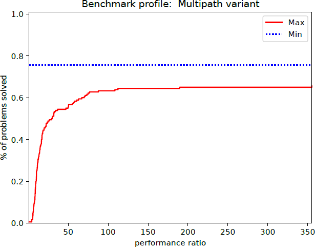
Finally, the benchmarking methodology proposed by Dolan & Moré (2002) is used to render Figure 1, in which the dominance of our minimization approach is further confirmed for the multiple path variant. Our minimization formulation is unequivocally superior in performance to its maximization counterpart.

Figure 1
Performance profile for the maximization and minimization formulations for the multiple path variant.

The benchmark profile graph by Dolan & Moré (2002), formally called performance profile, is a crucial methodological tool in the comparative analysis of numerical optimization solvers. It aims to provide an objective and robust assessment of the relative performance of a set of algorithms (S) on a battery of test problems (P), overcoming the limitations of simple aggregate metrics such as averages or totals.

The construction of the profile is based on the relative performance ratio τ _p,s , which compares the cost of a solver s on problem p (typically CPU time or number of iterations) with the best cost obtained by any solver for that same problem. The result is a cumulative distribution function, ρ _s (τ), which represents the probability that a solver s will solve a problem with a cost at most τ times higher than the best cost.

The interpretation of the performance profile reveals the efficiency and robustness characteristics of each solver. The intersection of the curve with the vertical axis at τ = 1 indicates absolute efficiency, denoting the fraction of problems for which the solver is the fastest (i.e., τ _p,s = 1). As the factor τ increases on the horizontal axis, the curve rises, indicating the robustness of the solver, which is the probability that it will solve a problem at a cost reasonably close to the minimum.

The curve that visually dominates the graph-being consistently higher and further to the left-is, by definition, representative of the superior solver, as it combines the highest probability of being the best solver (efficiency) with the highest likelihood of solving problems in general (robustness). Note that, when a solver fails to solve an instance, the benchmark profile methodology assigns an infinite performance ratio to that solver for that specific problem, implying thus that the solver is unable to solve that instance. For instance, a solver that fails on half of the problems will have its performance profile curve stopped at a maximum height of 0.5 on the y-axis. This is ensured by assigning an infinite performance ratio to the failed cases.

Table 3 presents the computational results for the single-path problem introduced by Tiwari et al. (2021b). The table has the same display structure as the previous one. Note that the results also show a similar trend. For problem sizes ranging from 10 to 30, our minimization formulation performs better than its maximization counterpart, presenting slightly inferior performance in only six cases out of 150.

Table 3
This table presents a comparison of the performance of the algorithms in solving instances with sizes n = {10, 15, 20, 25, 30, 40} while varying parameters p and α accordingly. We have included the average running times in seconds (cpu), the total count of branch-and-bound nodes (#bbn), and the final gaps.

n	p	α	Market share (%)	Singlepath original variant
					Maximization			Minimization
				cpu (s)	gap (%)	#bbn	cpu (s)/ratio	gap (%)	#bbn
		0.1	53.50	2.00		3	0.59/ 3.39		4
		0.2	53.67	6.09		3	0.94/ 6.48		3
		0.3	53.82	2.19		4	1.11/ 1.97		3
		0.4	53.97	6.91		3	1.08/ 6.40		3
	2	0.5	54.12	2.13		4	1.00/ 2.13		3
		0.6	54.03	1.91		8	0.56/ 3.41		3
		0.7	54.19	2.18		5	0.95/ 2.29		5
		0.8	54.07	5.86		5	0.87/ 6.74		3
		0.9	54.03	2.11		4	0.63/ 3.35		3
		1.0	53.93	15.34		3	0.86/ 17.84		3
		averages		4.67		4.20	0.86/ 5.44		3.30
		0.1	53.86	5.15		5	1.12/ 4.60		6
		0.2	54.22	4.76		5	0.50/ 9.52		5
		0.3	54.54	1.66		3	1.08/ 1.54		1
		0.4	54.90	1.56		3	0.55/ 2.84		1
	3	0.5	54.71	5.39		3	1.02/ 5.28		1
10		0.6	54.83	14.15		7	0.82/ 17.26		1
		0.7	55.16	5.53		3	1.20/ 4.61		3
		0.8	55.47	6.15		3	1.15/ 5.35		3
		0.9	54.83	14.09		7	0.96/ 14.68		3
		1.0	54.44	1.63		1	1.60/ 1.02		1
		averages		6.01		4.00	1.00/ 6.01		2.50
		0.1	54.95	4.46		10	0.54/ 8.26		6
		0.2	52.38	6.23		5	1.18/ 5.28		5
		0.3	51.41	2.01		5	0.69/ 2.91		4
		0.4	51.59	8.91		3	0.33/ 27.00		1
	4	0.5	51.73	1.85		2	0.43/ 4.30		1
		0.6	51.75	0.45		1	0.07/ 6.43		1
		0.7	51.96	0.45		1	0.54/ 0.83		1
		0.8	52.02	0.45		1	0.30/ 1.50		1
		0.9	51.95	0.44		1	0.26/ 1.69		1
		1.0	51.66	0.47		1	0.08/ 5.87		1
		averages		2.57		3.00	0.44/ 5.82		2.20
		0.1	52.56	20.86		1	2.53/ 8.25		1
		0.2	51.57	21.78		1	0.96/ 22.69		1
		0.3	51.07	20.94		1	0.86/ 24.35		1
		0.4	51.18	21.34		1	0.67/ 31.85		1
	2	0.5	50.48	20.76		1	0.93/ 22.32		1
		0.6	50.55	21.14		1	0.78/ 27.10		1
		0.7	50.62	20.64		1	0.64/ 32.25		1
		0.8	50.69	19.81		1	0.67/ 29.57		1
		0.9	50.76	21.34		1	0.72/ 29.64		1
		1.0	50.73	20.81		1	0.88/ 23.65		1
		averages		20.94		1.00	0.96/ 21.72		1.00
		0.1	53.20	65.12		5	6.35/ 10.26		3
		0.2	52.34	57.10		3	7.91/ 7.22		3
		0.3	51.93	62.50		5	7.08/ 8.83		3
		0.4	52.07	56.67		3	8.77/ 6.46		1
	3	0.5	51.49	66.62		5	6.47/ 10.30		3
15		0.6	51.64	243.70		17	10.18/ 23.94		5
		0.7	51.81	19.64		9	10.39/ 1.89		5
		0.8	51.97	64.02		5	3.12/ 20.52		6
		0.9	52.11	61.80		6	13.32/ 4.64		5
		1.0	52.03	271.16		18	3.72/ 72.89		13
		averages		96.83		7.60	7.73/ 12.53		4.70
		0.1	53.04	37.16		13	6.23/ 5.96		9
		0.2	51.80	13.85		17	6.53/ 2.12		10
		0.3	52.16	150.58		19	8.54/ 17.63		9
		0.4	52.58	31.00		16	8.85/ 3.50		11
	4	0.5	52.29	32.81		11	8.77/ 3.74		12
		0.6	52.70	147.13		19	8.38/ 17.56		16
		0.7	53.12	137.37		20	12.51/ 10.98		13
		0.8	53.37	47.85		13	7.98/ 6.00		11
		0.9	53.74	51.57		20	5.69/ 9.06		16
		1.0	53.44	63.03		11	7.46/ 8.45		14
		averages		71.23		15.90	8.09/ 8.80		12.10
		0.1	51.87	131.94		1	4.56/ 28.93		1
		0.2	51.97	137.07		1	3.93/ 34.88		1
		0.3	51.75	157.56		1	3.55/ 44.38		1
		0.4	51.55	150.93		1	4.16/ 36.28		1
	2	0.5	51.63	150.12		1	6.40/ 23.46		1
		0.6	51.42	150.11		1	5.07/ 29.61		1
		0.7	51.02	130.93		1	4.40/ 29.76		1
		0.8	51.08	143.80		1	3.56/ 40.39		1
		0.9	50.91	137.38		1	13.73/ 10.01		1
		1.0	50.69	144.29		1	2.64/ 54.66		1
		averages		143.41		1.00	5.20/ 27.58		1.00
		0.1	52.43	110.83		1	2.62/ 42.30		1
		0.2	52.59	91.67		1	3.51/ 26.12		1
		0.3	52.45	116.72		1	3.22/ 36.25		1
		0.4	52.34	103.61		1	2.63/ 39.40		1
	3	0.5	52.49	104.14		1	2.44/ 42.68		1
20		0.6	52.37	110.58		1	2.01/ 55.01		1
		0.7	52.06	111.51		1	2.05/ 54.40		1
		0.8	52.21	105.16		1	2.08/ 50.56		1
		0.9	52.07	98.44		1	10.90/ 9.03		1
		1.0	51.88	98.69		1	3.73/ 26.46		1
		averages		105.13		1.00	3.52/ 29.88		1.00
		0.1	54.21	223.35		3	27.97/ 7.99		1
		0.2	54.30	235.86		3	48.87/ 4.83		4
		0.3	53.99	208.30		6	6.07/ 34.32		7
		0.4	54.28	606.35		13	43.76/ 13.86		7
	4	0.5	54.14	68.91		4	31.73/ 2.17		3
		0.6	54.39	83.40		5	18.42/ 4.53		5
		0.7	54.67	90.82		4	35.15/ 2.58		5
		0.8	54.91	1001.71		15	15.57/ 64.34		5
		0.9	54.97	550.68		16	21.13/ 26.06		3
		1.0	54.63	84.10		4	23.42/ 3.59		1
		averages		315.35		7.30	27.21/ 11.59		4.10
		0.1	51.69	507.88		3	136.93/ 3.71		3
		0.2	51.78	440.73		3	105.21/ 4.19		3
		0.3	51.64	536.61		3	184.30/ 2.91		3
		0.4	51.47	483.04		3	208.95/ 2.31		3
	2	0.5	51.55	483.89		3	246.28/ 1.96		3
		0.6	51.36	503.77		3	192.83/ 2.61		3
		0.7	51.05	511.83		3	232.15/ 2.20		3
		0.8	51.11	516.18		3	181.92/ 2.84		3
		0.9	51.01	497.86		3	250.95/ 1.98		3
		1.0	50.88	164.86		1	149.02/ 1.11		3
		averages		464.66		2.80	188.85/ 2.46		3.00
		0.1	52.82	137.73		1	129.60/ 1.06		1
		0.2	52.80	106.55		1	12.17/ 8.76		1
		0.3	52.94	137.70		1	10.92/ 12.61		1
		0.4	52.90	135.01		1	11.98/ 11.27		1
	3	0.5	53.03	114.39		1	44.92/ 2.55		1
25		0.6	53.15	138.03		1	44.97/ 3.07		1
		0.7	53.29	128.59		1	9.34/ 13.77		1
		0.8	53.35	129.36		1	6.44/ 20.09		1
		0.9	53.41	133.10		1	9.53/ 13.97		1
		1.0	53.25	110.72		1	6.74/ 16.43		1
		averages		127.12		1.00	28.66/ 4.44		1.00
		0.1	53.92	77.75		1	124.10/ 0.63		1
		0.2	53.79	97.12		1	94.40/ 1.03		1
		0.3	53.99	93.02		1	16.23/ 5.73		1
		0.4	54.02	97.94		1	57.85/ 1.69		1
	4	0.5	53.97	94.56		1	45.71/ 2.07		1
		0.6	54.14	105.38		1	170.02/ 0.62		2
		0.7	54.32	88.13		1	125.88/ 0.70		3
		0.8	54.42	94.29		1	61.49/ 1.53		3
		0.9	54.48	74.84		1	139.34/ 0.54		1
		1.0	54.32	94.09		1	73.89/ 1.27		1
		averages		91.71		1.00	90.89/ 1.01		1.50
		0.1	63.10	3570.59	0.58	19	576.42/ 6.19		21
		0.2	60.84	2163.45		25	641.42/ 3.37		20
		0.3	59.92	3010.35		46	599.89/ 5.02		28
		0.4	58.85	2095.88		36	573.92/ 3.65		33
	4	0.5	58.46	1944.17		48	617.91/ 3.15		45
		0.6	58.38	968.45		39	709.44/ 1.37		32
		0.7	58.15	3572.27	0.63	16	621.51/ 5.75		49
		0.8	57.93	2754.42		33	615.91/ 4.47		41
		0.9	57.90	2434.51		33	646.07/ 3.77		38
		1.0	57.64	959.18		29	715.47/ 1.34		40
		averages		2347.33	0.12	32.40	631.80/ 3.72		34.70
		0.1	62.83	3532.04		8	829.51/ 4.26		3
		0.2	62.30	1737.08		3	744.17/ 2.33		3
		0.3	61.31	3557.55	0.03	6	563.50/ 6.31		5
		0.4	60.66	3538.28	0.05	8	832.53/ 4.25		6
	5	0.5	60.06	3571.21	0.02	9	908.93/ 3.93		9
30		0.6	59.60	3566.26	0.06	12	822.69/ 4.33		9
		0.7	59.25	859.66		8	961.54/ 0.89		16
		0.8	58.99	3551.29	0.05	7	829.18/ 4.28		9
		0.9	58.74	3572.17	0.14	11	1500.91/ 2.38		18
		1.0	58.13	3566.28		9	873.45/ 4.08		11
		averages		3105.18	0.04	8.10	886.64/ 3.50		8.90
		0.1	58.21	558.50		1	548.63/ 1.02		1
		0.2	57.68	601.82		1	139.27/ 4.32		1
		0.3	54.84	3490.19	3.84	3	531.49/ 6.57		1
		0.4	55.41	666.46		1	516.81/ 1.29		1
	6	0.5	52.99	3517.81	3.90	4	877.46/ 4.01		6
		0.6	54.42	2370.92		24	891.90/ 2.66		20
		0.7	53.96	3571.32	0.12	11	804.74/ 4.44		23
		0.8	54.08	-	-	-	1851.50/ -		22
		0.9	54.26	-	-	-	1380.79/ -		29
		1.0	52.77	3575.16	0.22	18	820.73/ 4.36		22
		averages		2294.02	1.01	7.88	836.33/ 2.74		12.60
		0.1	60.42	-	-	-	3352.13/ -	0.30	17
		0.2	59.83	3531.67	0.27	17	3350.42/ 1.05	0.64	10
		0.3	59.73	3542.75	0.46	1	3307.22/ 1.07		28
		0.4	59.48	-	-	-	3347.31/ -	0.58	17
	4	0.5	58.15	-	-	-	3358.11/ -	0.43	12
		0.6	-	-	-	-	-/ -	-	-
		0.7	-	-	-	-	-/ -	-	-
		0.8	-	-	-	-	-/ -	-	-
		0.9	-	-	-	-	-/ -	-	-
		1.0	-	-	-	-	-/ -	-	-
		averages		3537.21	0.36	9.00	3343.04/ 1.06	0.39	16.80
		0.1	64.60	-	-	-	3336.17/ -	0.02	13
		0.2	64.07	-	-	-	3354.22/ -	0.05	5
		0.3	63.78	-	-	-	3339.51/ -	0.05	6
		0.4	62.42	3541.72	0.08	1	3338.90/ 1.06	0.13	1
	5	0.5	61.86	-	-	-	3322.37/ -	0.05	6
40		0.6	-	-	-	-	-/ -	-	-
		0.7	-	-	-	-	-/ -	-	-
		0.8	-	-	-	-	-/ -	-	-
		0.9	-	-	-	-	-/ -	-	-
		1.0	59.95	-	-	-	3324.77/ -	0.11	9
		averages		3541.72	0.08	1.00	3335.99/ 1.06	0.07	6.67
		0.1	63.37	3539.77	0.17	1	3364.05/ 1.05	0.14	4
		0.2	61.30	-	-	-	3334.06/ -	0.12	10
		0.3	58.54	-	-	-	3342.55/ -	0.17	1
		0.4	57.40	-	-	-	3340.20/ -	0.04	10
	6	0.5	57.06	-	-	-	3351.39/ -	0.17	1
		0.6	-	-	-	-	-/ -	-	-
		0.7	-	-	-	-	-/ -	-	-
		0.8	55.53	-	-	-	2997.39/ -		10
		0.9	-	-	-	-	-/ -	-	-
		1.0	-	-	-	-	-/ -	-	-
		averages		3539.77	0.17	1.00	3288.27/ 1.08	0.11	6.00

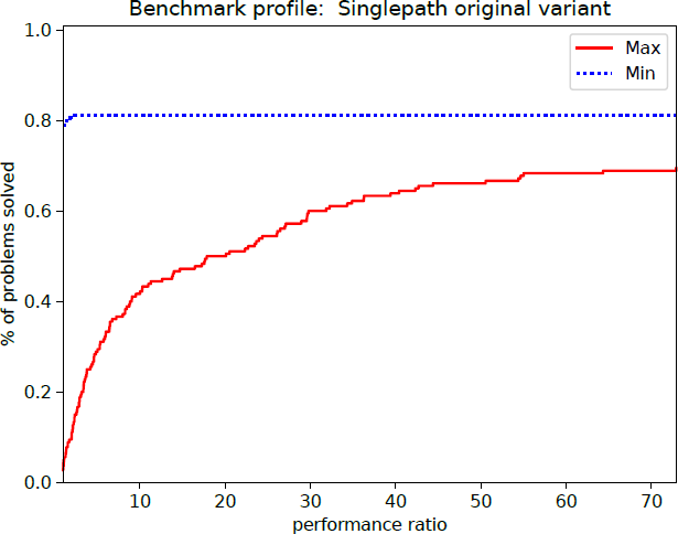
For instances with 40 nodes, our minimization model was able to optimally solve or return small optimality gaps for 17 of the 30 instances, while the maximization model failed to solve 24 instances within the given time limit and returned small optimality gaps for the others. Nonetheless, the benchmark performance profile shown in Figure 2 leaves no doubt about the superiority of our minimization model. It is important to note that both the original single-path maximization and minimization models did not take into account the concerns raised by Marín et al. (2006) who pointed out that the Hamacher et al. (2004)’s formulation can redeem incorrect hub-and-spoke networks when constraints like (13)-(15) are not added to the formulation.

Figure 2
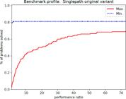
Performance profile for the maximization and minimization formulations for the single path original variant.

Hence, we have assessed the impact of these constraints on the single-path maximization and minimization models, reporting their computational results in Table 4. Recall that constraints (13)-(15) prevent the formation of pathological paths with more than two hubs on them. As can be seen in Table 4, these fixing constraints severely impact both formulations, substantially increasing the computational effort required to solve the same set of instances.

Table 4
This table presents a comparison of the performance of the algorithms in solving instances with sizes n = {10, 15, 20, 25, 30, 40} while varying parameters p and α accordingly. We have included the average running times in seconds (cpu), the total count of branch-and-bound nodes (#bbn), and the final gaps.

n	p	α	Market share (%)	Singlepath fixed variant
					Maximization			Minimization
				cpu (s)	gap (%)	#bbn	cpu (s)/ratio	gap (%)	#bbn
		0.1	53.34	3.84		4	0.90/ 4.27		3
		0.2	53.47	3.91		4	0.99/ 3.95		3
		0.3	53.59	11.88		3	1.02/ 11.65		3
		0.4	53.70	4.02		4	1.18/ 3.41		3
	2	0.5	53.81	3.71		5	1.12/ 3.31		3
		0.6	53.68	3.63		5	1.03/ 3.52		5
		0.7	53.76	9.41		5	0.58/ 16.22		5
		0.8	53.56	3.69		5	0.65/ 5.68		7
		0.9	53.44	4.02		8	0.86/ 4.67		3
		1.0	53.28	3.87		7	0.57/ 6.79		5
		averages		5.20		5.00	0.89/ 5.84		4.00
		0.1	53.78	14.86		4	1.35/ 11.01		5
		0.2	54.12	3.55		7	0.81/ 4.38		3
		0.3	54.43	3.55		3	0.67/ 5.30		1
		0.4	54.77	3.58		1	0.76/ 4.71		1
	3	0.5	54.57	3.72		1	1.08/ 3.44		1
10		0.6	54.67	3.62		1	1.18/ 3.07		1
		0.7	54.93	4.49		1	0.72/ 6.24		1
		0.8	55.18	3.71		1	1.39/ 2.67		1
		0.9	54.48	2.88		1	0.38/ 7.58		1
		1.0	54.06	4.31		1	0.98/ 4.40		1
		averages		4.83		2.10	0.93/ 5.18		1.60
		0.1	54.51	3.56		7	1.26/ 2.83		10
		0.2	51.90	3.73		5	1.12/ 3.33		5
		0.3	50.87	3.01		3	0.85/ 3.54		1
		0.4	50.85	7.48		3	0.83/ 9.01		3
	4	0.5	50.83	7.86		3	1.35/ 5.82		3
		0.6	50.68	16.61		5	0.88/ 18.88		5
		0.7	50.63	44.26		13	0.37/ 119.62		8
		0.8	50.45	12.50		9	0.60/ 20.83		6
		0.9	50.14	24.18		9	0.55/ 43.96		10
		1.0	49.60	4.40		11	0.90/ 4.89		15
		averages		12.76		6.80	0.87/ 14.65		6.60
		0.1	52.53	36.89		1	5.12/ 7.21		1
		0.2	51.52	38.23		1	1.13/ 33.83		1
		0.3	51.01	36.65		1	0.86/ 42.62		1
		0.4	51.10	35.46		1	1.04/ 34.10		1
	2	0.5	50.38	35.14		1	1.39/ 25.28		1
		0.6	50.42	32.80		1	1.97/ 16.65		1
		0.7	50.47	36.25		1	1.51/ 24.01		1
		0.8	50.52	35.38		1	1.47/ 24.07		1
		0.9	50.57	36.09		1	1.24/ 29.10		1
		1.0	50.52	36.73		1	0.57/ 64.44		1
		averages		35.96		1.00	1.63/ 22.06		1.00
		0.1	53.09	134.53		5	12.13/ 11.09		5
		0.2	52.20	88.13		8	10.06/ 8.76		5
		0.3	51.73	127.12		3	9.40/ 13.52		3
		0.4	51.81	144.17		6	13.05/ 11.05		5
	3	0.5	51.21	172.25		8	12.07/ 14.27		5
15		0.6	51.35	108.84		8	11.02/ 9.88		5
		0.7	51.48	135.32		6	14.04/ 9.64		7
		0.8	51.59	322.68		14	14.24/ 22.66		5
		0.9	51.69	424.69		15	8.98/ 47.29		5
		1.0	51.57	116.91		6	9.58/ 12.20
		averages		177.46		7.90	11.46/ 15.49		5.00
		0.1	52.71	105.99		10	8.10/ 13.09		12
		0.2	51.43	363.18		38	7.74/ 46.92		26
		0.3	51.80	517.65		36	8.97/ 57.71		23
		0.4	52.18	111.04		20	2.38/ 46.66		18
	4	0.5	51.85	74.63		18	1.95/ 38.27		20
		0.6	52.20	370.05		31	10.37/ 35.68		15
		0.7	52.53	123.74		17	12.21/ 10.13		16
		0.8	52.68	33.46		23	3.37/ 9.93		21
		0.9	52.97	111.81		27	8.84/ 12.65		20
		1.0	52.61	107.41		25	5.13/ 20.94		26
		averages		191.90		24.50	6.91/ 27.79		19.70
		0.1	51.78	247.30		1	4.07/ 60.76		1
		0.2	51.85	236.08		1	6.84/ 34.51		1
		0.3	51.61	242.26		1	17.04/ 14.22		1
		0.4	51.41	240.38		1	4.49/ 53.54		1
	2	0.5	51.48	231.71		1	8.83/ 26.24		1
		0.6	51.25	219.55		1	4.28/ 51.30		1
		0.7	50.83	234.19		1	4.00/ 58.55		1
		0.8	50.88	239.89		1	5.96/ 40.25		1
		0.9	50.68	241.88		1	5.49/ 44.06		1
		1.0	50.44	233.43		1	1.90/ 122.86		1
		averages		236.67		1.00	6.29/ 37.63		1.00
		0.1	52.29	131.43		1	5.29/ 24.84		1
		0.2	52.42	132.63		1	5.19/ 25.55		1
		0.3	52.26	135.59		1	15.07/ 9.00		1
		0.4	52.11	244.55		1	7.94/ 30.80		1
	3	0.5	52.24	242.92		1	6.07/ 40.02		1
20		0.6	52.09	225.41		1	12.27/ 18.37		1
		0.7	51.73	243.18		1	3.81/ 63.83		1
		0.8	51.83	132.66		1	5.21/ 25.46		1
		0.9	51.63	123.95		1	4.62/ 26.83		1
		1.0	51.39	125.60		1	4.06/ 30.94		1
		averages		173.79		1.00	6.95/ 25.00		1.00
		0.1	53.97	422.58		10	46.80/ 9.03		3
		0.2	54.04	479.20		12	36.66/ 13.07		13
		0.3	53.74	430.52		5	31.51/ 13.66		8
		0.4	53.99	481.10		5	29.95/ 16.06		5
	4	0.5	53.79	1042.43		11	17.26/ 60.40		5
		0.6	53.99	450.42		5	23.26/ 19.36		5
		0.7	54.17	3363.53		23	28.98/ 116.06		6
		0.8	54.33	2194.98		17	73.75/ 29.76		4
		0.9	54.31	432.14		6	54.11/ 7.99		6
		1.0	53.91	135.37		5	49.11/ 2.76		7
		averages		943.23		9.90	39.14/ 24.10		6.20
		0.1	51.62	652.79		3	184.24/ 3.54		3
		0.2	51.70	494.86		3	180.93/ 2.74		3
		0.3	51.55	1957.70		3	237.69/ 8.24		3
		0.4	51.36	1604.06		3	240.02/ 6.68		3
	2	0.5	51.43	1047.58		3	194.89/ 5.38		3
		0.6	51.23	1845.94		3	301.47/ 6.12		3
		0.7	50.90	1168.14		3	266.04/ 4.39		3
		0.8	50.96	1780.53		2	159.50/ 11.16		3
		0.9	50.84	1105.34		2	351.02/ 3.15		3
		1.0	50.70	185.38		1	132.45/ 1.40		3
		averages		1184.23		2.60	224.82/ 5.27		3.00
		0.1	52.65	144.13		1	152.05/ 0.95		1
		0.2	52.61	120.75		1	123.54/ 0.98		1
		0.3	52.71	164.33		1	52.81/ 3.11		1
		0.4	52.65	133.11		1	51.17/ 2.60		1
	3	0.5	52.75	121.56		1	54.94/ 2.21		1
25		0.6	52.85	145.18		1	60.50/ 2.40		1
		0.7	52.94	165.61		1	17.91/ 9.25		1
		0.8	52.96	144.78		1	11.92/ 12.15		1
		0.9	52.99	133.51		1	49.78/ 2.68		1
		1.0	52.79	121.53		1	50.13/ 2.42		1
		averages		139.45		1.00	62.48/ 2.23		1.00
		0.1	53.70	101.07		1	50.79/ 1.99		1
		0.2	53.52	96.93		1	19.45/ 4.98		1
		0.3	53.68	84.67		1	146.66/ 0.58		1
		0.4	53.65	98.84		1	49.23/ 2.01		1
	4	0.5	53.54	127.89		1	131.33/ 0.97		1
		0.6	53.65	115.68		1	180.23/ 0.64		1
		0.7	53.75	125.13		1	153.73/ 0.81		1
		0.8	53.77	117.76		1	147.05/ 0.80		3
		0.9	53.75	116.49		1	187.25/ 0.62		1
		1.0	53.52	843.89		3	128.26/ 6.58		5
		averages		182.83		1.20	119.40/ 1.53		1.60
		0.1	63.10	3594.62	0.62	18	595.74/ 6.03		25
		0.2	60.84	646.57		24	604.54/ 1.07		24
		0.3	59.92	3672.54	0.65	18	623.72/ 5.89		27
		0.4	58.85	652.46		39	597.57/ 1.09		25
	4	0.5	58.46	3613.26	0.10	42	550.79/ 6.56		37
		0.6	58.38	3705.99	0.07	33	729.56/ 5.08		40
		0.7	58.09	3584.75	0.65	8	833.78/ 4.30		45
		0.8	57.65	3704.97	0.93	14	678.19/ 5.46		31
		0.9	57.49	3784.34	1.05	26	836.22/ 4.53		37
		1.0	57.45	3681.44	0.30	8	691.13/ 5.33		15
		averages		3064.09	0.44	23.00	674.12/ 4.55		30.60
		0.1	62.83	1258.10		3	781.70/ 1.61		3
		0.2	62.30	3561.09	0.04	8	814.12/ 4.37		3
		0.3	61.31	3752.46	0.08	3	557.98/ 6.73		1
		0.4	60.66	3965.19	0.05	3	677.87/ 5.85		6
	5	0.5	60.06	3573.08	0.02	10	804.31/ 4.44		5
30		0.6	59.60	4122.74		7	626.07/ 6.59		6
		0.7	59.05	3694.36	0.31	7	787.27/ 4.69		15
		0.8	58.49	3748.25	0.53	6	1093.05/ 3.43		14
		0.9	58.02	3803.90	0.84	14	896.77/ 4.24		12
		1.0	57.23	3559.03	0.73	9	749.80/ 4.75		16
		averages		3503.82	0.26	7.00	778.89/ 4.50		8.10
		0.1	58.21	484.88		1	530.18/ 0.91		1
		0.2	57.68	495.56		1	107.95/ 4.59		1
		0.3	56.94	483.95		1	505.26/ 0.96		1
		0.4	55.41	1801.07		1	540.29/ 3.33		1
	6	0.5	55.06	3601.94	0.03	4	600.13/ 6.00		6
		0.6	54.15	3852.20	0.56	11	922.81/ 4.17		20
		0.7	53.62	3547.73	0.53	6	1065.65/ 3.33		7
		0.8	52.07	3547.72	3.49	8	1650.56/ 2.15		19
		0.9	52.00	3539.50	3.41	4	1915.49/ 1.85		17
		1.0	52.15	3554.13	0.77	10	1423.24/ 2.50		7
		averages		2490.87	0.88	4.70	926.16/ 2.69		8.00
		0.1	60.42	3512.96		31	3343.42/ 1.05	0.51	10
		0.2	59.83	3481.57		26	3276.29/ 1.06		14
		0.3	59.73	3478.74		29	3294.60/ 1.06		26
		0.4	59.48	3542.12	0.40	1	3060.77/ 1.16		27
	4	0.5	58.15	3540.90	0.28	18	3261.58/ 1.09		27
		0.6	-	-	-	-	-/ -	-	-
		0.7	57.20	-	-	-	3351.50/ -	0.85	1
		0.8	56.69	-	-	-	3357.64/ -	0.41	22
		0.9	-	-	-	-	-/ -	-	-
		1.0	56.20	-	-	-	3168.83/ -		39
		averages		3511.26	0.14	21.00	3264.33/ 1.08	0.22	20.75
		0.1	64.60	3154.35		15	3341.21/ 0.94	0.28	10
		0.2	64.07	-	-	-	3368.01/ -	0.05	5
		0.3	63.78	3307.36		7	3043.42/ 1.09		7
		0.4	62.42	3532.45	0.06	7	3318.88/ 1.06	0.07	7
	5	0.5	61.86	5046.15	0.06	8	-/ -	-	-
40		0.6	-	-	-	-	-/ -	-	-
		0.7	-	-	-	-	-/ -	-	-
		0.8	-	-	-	-	-/ -	-	-
		0.9	59.61	-	-	-	3341.62/ -	0.69	1
		1.0	59.28	-	-	-	3359.70/ -	1.00	1
		averages		3760.08	0.03	9.25	3295.47/ 1.14	0.35	5.17
		0.1	63.37	3525.68		13	-/ -	-	-
		0.2	61.30	3070.18		13	3345.75/ 0.92	0.07	11
		0.3	58.54	3436.42		11	3339.89/ 1.03	0.04	10
		0.4	57.40	3541.63	0.03	10	3330.06/ 1.06	0.04	8
	6	0.5	57.06	3566.42	0.03	10	3373.27/ 1.06	0.17	1
		0.6	-	-	-	-	-/ -	-	-
		0.7	55.49	3542.35	0.16	1	-/ -	-	-
		0.8	55.12	-	-	-	3342.29/ -	0.42	1
		0.9	-	-	-	-	-/ -	-	-
		1.0	54.44	-	-	-	3355.02/ -	0.57	15
		averages		3447.11	0.04	9.67	3347.71/ 1.03	0.22	7.67

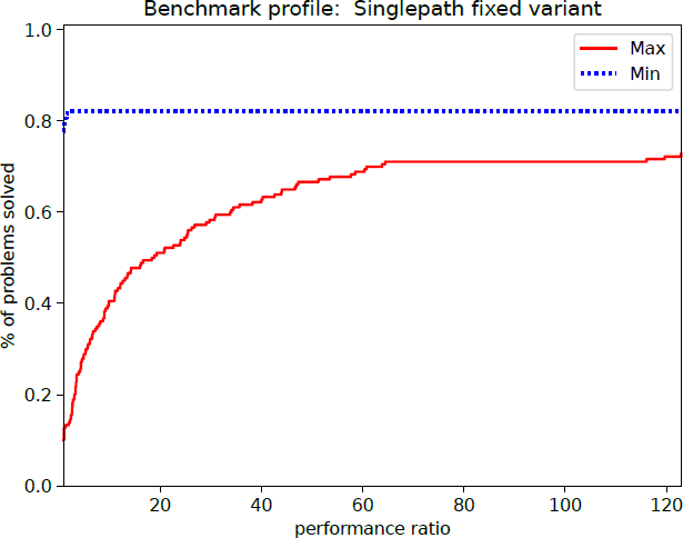
On the one hand, Tiwari et al. (2021b)’s formulation performance seems to be more affected for problem sizes ranging from 10 to 30, with the impact being more pronounced for the latter size, as the established time limit is reached more often before finding an optimal solution. On the other hand, analyzing the 40 node instances, it is hard to define a winning model, as both seem to be tied. Unfortunately, this effect is not observed in the performance profile shown in Figure 3, as it clearly favors our minimization model.

Figure 3
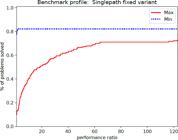
Performance profile for the maximization and minimization formulations for the single path fixed variant.

One may argue that the given time limit may interfere with the results, especially for p = 5, p = 6, and n = 40, since these results do not clearly differ from one model to the other, making it hard to declare a winning model. Therefore, we have designed an additional computational experiment in which we have removed the imposition of a time limit while solving an instance with n = 50 and p = 5. The idea is to break the ties and further investigate both behavior of both formulations’ without the interference of a time limit while addressing larger problems.

Table 5 reports the attained results. While clearly demonstrating the dominance of the minimization model once again, since the maximization model of Tiwari et al. (2021b) fails to render bounds for all instances due to a lack of memory, meaning that it would take more than 256 GB of RAM to run the model properly, our minimization formulation was able to reach proven optimality for all instances in under 6.5 hours.

Table 5
This table presents a comparison of the performance of the algorithms in solving instances with size n = {50} with parameter p = 5 and parameter varying α accordingly. All time limits removed. We have included the average running times in seconds (cpu), the total count of branch-and-bound nodes (#bbn), and the final gaps.

n	p	α	Market share (%)	Singlepath fixed variant
					Maximization			Minimization
				cpu (s)	gap (%)	#bbn	cpu (s)/ratio	gap (%)	#bbn
		0.1	57.83	-	-	-	21542.38 / -		5
		0.2	56.99	-	-	-	21325.03 / -		5
		0.3	56.94	-	-	-	13546.64 / -		2
		0.4	56.85	-	-	-	17051.10 / -		3
50	5	0.5	56.45	-	-	-	13178.33 / -		2
		0.6	56.09	-	-	-	23218.64 / -		4
		0.7	55.66	-	-	-	19803.84 / -		7
		0.8	54.76	-	-	-	17322.16 / -		13
		0.9	54.30	-	-	-	20095.53 / -		24
8		1.0	53.76	-	-	-	17371.56 / -		26
		averages		-	-	-	18446.52 / -		9.1

Please recall the highlighted difference between empty entries versus entries marked with ’-’, when not even the continuous bounds are available. Nevertheless, it could be argued that the new formulations are still very resource-intensive, considering the memory usage and the solution times achieved. This is a clear indication that the proposed formulations would require a decomposition effort in order to improve their scalability. This might be a direction for future research, provided that for a fixed hub structure, the origin-destination pairwise decomposition is preserved by constraints (13) - (15), easily allowing for a Benders’ decomposition scheme, for instance.

5 CONCLUSION AND FINAL REMARKS

In conclusion, our proposed models offer a simpler, more robust, and efficient approach to both problem variants with single and multiple paths, outperforming the previous models proposed by Tiwari et al. (2021a) and Tiwari et al. (2021b). Instead of maximizing the market share of an entrant company, we have adopted the strategy of minimizing the loss of market share. This has represented a significant advancement over traditional assumptions.

Future research could explore more advanced methodologies for handling large-scale problems, such as the generalized Benders Decomposition (Geoffrion, 1972; de Camargo et al., 2009; Miranda Jr et al., 2011; Miranda Jr. et al., 2011; de Camargo & Miranda Jr, 2012; de Camargo & Miranda, 2012) or the Outer Approximation technique combined with the Benders’ Decomposition method (de Camargo et al., 2011) to further improve solution efficiency. In addition, investigating sources of uncertainty in problem data, such as variability in transportation flows, could make the model more realistic and adaptable to practical scenarios.

Finally, despite the growing body of articles in this field, there is a lack of studies that include the topic of environmental sustainability as a factor in the attractiveness of the choice of transport. Furthermore, the present study have focused on a single-objective market-share formulation, but real-world hub-network design is inherently multi-objective. Investigating extensions that simultaneously maximize the captured flow, minimize transportation costs, carbon emissions, and embed richer user-preference models as a way to optimize service attractiveness represents a promising avenue for future research.

Acknowledgements

The authors thank CNPq for its financial support, grants 305478/2022-2 and 423065/2021-1.

Data Availability

All the source codes and instances used to produce the results of this article are available in GitHub at https://github.com/risargo/MIQCPMAPHLP or in Open Science Framework (OSF) at https://osf.io/wq6jt/?view only=78700465d980479d897b6f8082740d21. The data might also be available from the authors upon request.

References

• ATAMTÜRK A, BERENGUER G & SHEN ZJ. 2012. A conic integer programming approach to stochastic joint location-inventory problems. Operations Research, 60(2): 366-381.
• BENTAL A & NEMIROVSKI A. 2001. Lectures on modern convex optimization: analysis, algorithms, and engineering applications. SIAM.
• BENSON HY & ÜMIT SAĞLAM. 2014. Mixed-Integer Second-Order Cone Programming: A Survey. chap. Chapter 2, pp. 13-36. Informs. Available at: https://pubsonline.informs.org/doi/abs/10.1287/educ.2013.0115
  » https://pubsonline.informs.org/doi/abs/10.1287/educ.2013.0115
• CAMPBELL JF & O’KELLY ME. 2012. Twenty-five years of hub location research. Transportation Science, 46(2): 153-169.
• CONTRERAS I & O’KELLY ME. 2019. Hub Location Problems. pp. 327-363. Cham: Springer International Publishing. Available at: https://doi.org/10.1007/978-3-030-32177-2_12
  » https://doi.org/10.1007/978-3-030-32177-2_12
• DE CAMARGO RS, DE MIRANDA JR G & FERREIRA RP. 2011. A hybrid outer-approximation/benders decomposition algorithm for the single allocation hub location problem under congestion. Operations Research Letters, 39(5): 329-337.
• DE CAMARGO RS & MIRANDA G. 2012. Single allocation hub location problem under congestion: Network owner and user perspectives. Expert Systems with Applications, 39(3): 3385-3391.
• DE CAMARGO RS & MIRANDA JR G. 2012. Addressing congestion on single allocation hub-and-spoke networks. Pesquisa Operacional, 32: 465-496.
• DE CAMARGO RS, MIRANDA JR G, FERREIRA RPM & LUNA H. 2009. Multiple allocation hub-and-spoke network design under hub congestion. Computers & Operations Research , 36(12): 3097-3106.
• DOLAN ED & MORÉ JJ. 2002. Benchmarking optimization software with performance profiles. Mathematical programming, 91: 201-213.
• DREZNER T & DREZNER Z. 2001. A Note on Applying the Gravity Rule to the Airline Hub Problem. Journal of Regional Science, 41(1): 67-72. Available at: https://onlinelibrary.wiley.com/doi/abs/10.1111/0022-4146.00207
  » https://onlinelibrary.wiley.com/doi/abs/10.1111/0022-4146.00207
• EISELT HA & MARIANOV V. 2009. A conditional p-hub location problem with attraction functions. Computers & Operations Research , 36(12): 3128-3135.
• GEOFFRION A. 1972. Generalized Benders decomposition. Journal of Optimization Theory and Applications, 10: 237-260.
• HAMACHER HW, LABBÉ M, NICKEL S & SONNEBORN T. 2004. Adapting polyhedral properties from facility to hub location problems. Discrete Applied Mathematics, 145(1): 104-116. Available at: https://www.sciencedirect.com/science/article/pii/S0166218X04000691 graph Optimization IV.
  » https://www.sciencedirect.com/science/article/pii/S0166218X04000691
• HUFF DL. 1964. Defining and estimating a trading area. Journal of marketing, 28(3): 34-38.
• HUFF DL. 1966. A Programmed Solution for Approximating an Optimum Retail Location. Land Economics, 42(3): 293-303.
• MARÍN A, CÁNOVAS L & LANDETE M. 2006. New formulations for the uncapacitated multiple allocation hub location problem. European Journal of Operational Research, 172(1): 274-292. Available at: https://www.sciencedirect.com/science/article/pii/S0377221704007994
  » https://www.sciencedirect.com/science/article/pii/S0377221704007994
• MIRANDA JR G, DE CAMARGO RS, PINTO LR, CONCEIÇÃO SV & FERREIRA RPM. 2011. Hub location under hub congestion and demand uncertainty: the Brazilian case study. Pesquisa Operacional , 31: 319-349.
• MIRANDA JR G, LUNA HPL, DE CAMARGO RS & PINTO LR. 2011. Tree network design avoiding congestion. Applied mathematical modelling, 35(9): 4175-4188.
• O’KELLY ME. 1986. The location of interacting hub facilities. Transportation science, 20(2): 92-106.
• O’KELLY ME. 1987. A quadratic integer program for the location of interacting hub facilities. European journal of operational research, 32(3): 393-404.
• O’KELLY ME & BRYAN D. 1998. Hub location with flow economies of scale. Transportation research part B: Methodological, 32(8): 605-616.
• TIWARI R, JAYASWAL S & SINHA A. 2021a. Alternate solution approaches for competitive hub location problems. European Journal of Operational Research, 290: 68-80.
• TIWARI R, JAYASWAL S & SINHA A. 2021b. Competitive hub location problem: Model and solution approaches. Transportation research part B: Methodological , 146: 237-261.

Edited by

• Editor responsible for the review
  Editor-in-Chief: Annibal Parracho Sant’Anna.

Publication Dates

• Publication in this collection
  06 Feb 2026
• Date of issue
  2026

History

• Received
  02 July 2025
• Accepted
  02 Nov 2025