AN EFFICIENT COUNT DATA MODEL: PROPERTIES, ACTUARIAL MEASURES, BAYESIAN ESTIMATION, REGRESSION MODEL, AND APPLICATIONS TO HEALTH CARE DATA

ABSTRACT

Based on the compounding mechanism, a unique discrete probability distribution is investigated in this paper. The Poisson distribution is mixed with a lifetime model called as the Fav-Jerry model. The important statistical properties are investigated and inferred. Further, the Actuarial measures have also been studied. The Bayesian estimation approach and the maximum likelihood method are used for the estimation process. Using a Monte-Carlo simulation technique, the behavior of the maximum likelihood estimate is examined. Additionally, when data is reproduced from different competing models, the model compatibility is being examined. The study further introduces a novel count data regression model for overdispersed data by assuming that the response variable follows the Poisson mixture of Fav-Jerry model. Various performance criteria are considered and real-world data sets are used to investigate the model’s applicability in real life. The outcomes are juxtaposed with few potentially intriguing models. The real world application of the regression model is also investigated.

Keywords:
Poisson mixture; bayesian estimation; count regression

1 INTRODUCTION

Since its inception, distribution theory has evolved considerably, with recent developments placing greater emphasis on addressing practical challenges faced by practitioners and applied researchers, while also introducing a range of techniques for effective data analysis and interpretation. To put it another way, there is a critical need to create useful models for better investigation of real occurrences. Utilizing count data analysis to comprehend the recurrence of occurrences in the actual world is a good illustration of this. The applications of distribution theory extend far beyond the field of Statistics and can be found in a wide range of fields. In the discipline of probability theory, there exist numerous discrete distributions with specifically stated applications. There is a widespread use of Poisson and Negative-Binomial models while dealing with count data starting from zero. In the former, the variance equals the mean, whereas in the latter, the variance exceeds the mean, indicating over-dispersion. At times, we notice emerging patterns in our count data that these models are unable to fully explain. To get around these limitation and to be employed in situations where standard distributions don’t provide a good match, researchers typically develop new probability distributions. Developing novel probability distributions to handle data that are poorly fit by conventional parametric distributions can be done in a sound and inventive way by using various well-known techniquesPoisson mixture modeling, Discretization, Zero-Inflation etc. When a random variable follows a distribution whose parameter (s) is itself a random variable, the consequential model produced is referred to as compound probability distribution.

Researchers have been studying this topic of statistical modeling since 1920 because of techniques applicability in so many domains. In a study conducted by Greenwood & Yule (1920), they made an important observation. They found that by expressing the rate parameter in the Poisson distribution (PD) as a Gamma variate, they identified a means that related the PD to the Negative-Binomial distribution (NBD). By compounding the PD with the Lindley distribution, Sankaran (1970) put forth the compound PD. The piece of writing provided illustrations of fitting real data and matched up the fit acquired to fits obtained by means of other distributions. Zamani (2010) introduced a novel mixed Negative-Binomial distribution by combining it with Lindley distribution. Using this newly developed model, they applied it to analyze insurance data in two distinct sample sets. By analyzing the inspiration, early contributions, and seminal accomplishments of probability models for over-dispersion as well as their effect and practical application, Xekalaki (2014) gave a historical perspective on the field. Tahir & Cordeiro (2016) made on hand a review of the literature on the subject of compound univariate distributions, as well as a debate on their extension and classes. The Poisson-Akash distribution (PAD) was devised by Shanker (2016) based on the compounding mechanism. The real life applicability of PAD was illustrated by employing data sets from the fields of Ecology, Genetics etc. A new one-parameter Poisson mixture of Bilal distribution was put forward by Altun (2020). He also developed the associated regression and integer-valued autoregressive model. Hassan et al. (2020) developed a new flexible discrete distribution with applications to count data by compounding the Poisson and the Ailamujia distribution [7]. Recently, Seghier & Zeghdoudi (2021) developed the Poisson XLindley distribution with applications. The validity of compound distributions was experienced by Goffard et al. (2022) by employing the goodness-of-fit methodologies. One of the recent works in this field is by Ahmad & Wani (2023). They compounded the Poisson distribution with Chrisjerry distribution and proved the real life applicability of the model using four real life data sets. The zero-inflated Poisson distribution was compounded with the Akash distribution by Wani & Ahmad (2023) to develop a novel compound model for handling zero-inflation in count data.

In spite of the reality that a lot of advancement has been made in these areas of distribution theory, there is always a requirement for new models to be put forward. Our goal is to extensively study a versatile probability distribution put forward by Irshad et al. (2024). Not only this, we are also going to devise the regression model of the same for the purpose of count data regression modeling. The different trends that come into sight in our count data on a usual basis are the encouragement for these models.

Ekemezie & Obulezi (2024) have proposed the Fav-Jerry distribution (FJD), a unique lifetime distribution. The formula for the FJD is a mixture of a gamma distribution with shape and scale parameter 2 and α, respectively, and an exponential distribution with scale parameter α, where $\frac{2}{{\alpha }^2+2}$ is the mixing proportion. Here is the FJD probability density function.

$f(x;\alpha )=\frac{\alpha }{2+{\alpha }^2}(2+{\alpha }^{3}x)e^{-\alpha x};x>0,\alpha >0.$ (1)

We study a flexible discrete distribution by combining the Poisson and FJD. The recommended distribution is predicted to perform best with over-dispersed count data due to its over-dispersed character. The study’s structure is as follows. The Section 2 provides the derivation of the model along with some study of the shape of model. In Section 3 several properties of the model are put forward. In Section 4, the procedure of the estimation of parameter is carried out. The MonteCarlo Simulation study is given in Section 5. The real-world applicability is discussed in Section 6. The novel count data regression model introduced in this study along with its real life application is presented in the Section 7. The study’s conclusion is given in Section 8.

2 POISSON-MIXTURE MODEL

A Poisson mixture of FJD is the distribution that results if the Poisson distribution’s parameter λ follows FJD (1). This mixture, which has the following probability mass function (PMF), is referred hereafter as PFJD.

$P(X=x)=\frac{\alpha }{2+{\alpha }^2}\left[\frac{{\alpha }^3(x+1)+2(1+\alpha )}{(1+\alpha {)}^{x+2}}\right];x=0,1,2,...,\alpha >0.$ (2)

Proof 1. This serves as proof of the outcome (2)

$$\begin{gathered} P(X=x)={\int }_0^{\infty }\frac{e^{-\lambda }{\lambda }^x}{x!}\frac{\alpha }{2+{\alpha }^2}(2+{\alpha }^3\lambda )e^{-\alpha \lambda }d\lambda \\ =\frac{\alpha }{2+{\alpha }^2}\frac{1}{x!}{\int }_0^{\infty }{e}^{-(\alpha +1)\lambda }{\lambda }^x(2+{\alpha }^3\lambda )d\lambda \\ =\frac{\alpha }{2+{\alpha }^2}\left[\frac{{\alpha }^3(x+1)+2(1+\alpha )}{(1+\alpha {)}^{x+2}}\right];x=0,1,2,...,\alpha >0. \end{gathered}$$

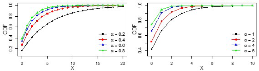
Remark 1. The corresponding Cumulative Distribution Function (CDF) of PFJD after some computations can be written as

$F_x\left(x\right)=1-\frac{2+2\alpha +{\alpha }^2+{\alpha }^3(x+2)}{(2+{\alpha }^2)(1+\alpha {)}^{x+2}}.$ (3)

Figure 1
PMF graphs of the PFJD for various parameter selections.

Figure 2
CDF plots of the PFJD for different parameter values.

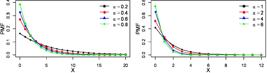
Remark 2: The Mean deviation (MD) of PFJD can be computed by using the results of Bakouch et al. (2014) as follows

$$\begin{gathered} \mathrm{MD}=2\mu F_x\left(\mu \right)-2\sum _{x=0}^{\mu }x\left\{\frac{\alpha }{2+{\alpha }^2}\left[\frac{{\alpha }^3(x+1)+2(1+\alpha )}{(1+\alpha {)}^{x+2}}\right]\right\} \\ \mathrm{MD}=2\mu F_x\left(\mu \right)-\frac{4\left[\right(1+\alpha {)}^{\mu }-1]+2\alpha (1+\alpha {)}^{\mu }[2+\alpha (2+\alpha (2+\alpha )\left)\right]-(2+\mu )\alpha [2+\alpha (2+\alpha (2+\alpha +\mu \alpha )\left)\right]}{\alpha (2+{\alpha }^2)(1+\alpha {)}^{2+\mu }}, \end{gathered}$$

where µ is the mean of PFJD and F _x (µ) can be calculated from the CDF of PFJD itself.

Remark 3: The PFJD is log-concave.

Proof 2: To demonstrate the log-concavity of the PFJD, it is enough to establish that:

$\left[P\right(X=x){]}^2\ge P(X=x-1)\bullet P(X=x+1)$

for α < 0 and x = 1, 2, 3, . . .

$\frac{{\alpha }^2}{(2+{\alpha }^2{)}^2}{\left[\frac{{\alpha }^3(x+1)+2(1+\alpha )}{(1+\alpha {)}^{x+2}}\right]}^2\ge \frac{{\alpha }^2}{(2+{\alpha }^2{)}^2}\left[\frac{{\alpha }^{3}x+2(1+\alpha )}{(1+\alpha {)}^{x+1}}\right]\left[\frac{{\alpha }^3(x+2)+2(1+\alpha )}{(1+\alpha {)}^{x+3}}\right],$

After some computations, we have ${\alpha }^8(1+\alpha {)}^{-2(2+x)}({\alpha }^2+2{)}^{-2}\ge 0$. This proves the log-concavity of PFJD.

Corollary 1: The following results hold as a direct consequence of log-concavity [see Keilson & Gerber (1971) and Bagnoli & Bergstrom (2005)]

• It has a unique mode.

• It is characterized by an increasing rate of hazard.

• The shape of its mean residual life function shows decreasing trend.

• All moments exist.

• It remains log-concave even if the model is truncated.

• The log-concavity holds even if the model is convoluted.

Remark 4: The Survival function refers to the likelihood that a system will survive past a specific point in time. More specifically, it examines the probability that a device would malfunction after a predetermined amount of time. It can be computed from the model’s CDF (3).

$S_x\left(x\right)=P(X>x)=\frac{2+2\alpha +{\alpha }^2+{\alpha }^3(x+2)}{(2+{\alpha }^2)(1+\alpha {)}^{x+2}}.$

Remark 5: A unit’s lifespan is monitored throughout its lifetime using the failure rate or Hazard rate. In actuality, it usually offers more details about the fundamental process of failure than the other representatives.

$h_x\left(x\right)=\frac{P(X=x)}{S_x\left(x\right)}=\frac{\alpha \left[{\alpha }^3\right(x+1)+2(1+\alpha \left)\right]}{2+2\alpha +{\alpha }^2+{\alpha }^3(x+2)}.$

Remark 6:h_x (x) is an increasing function of x.

Proof 3: Incorporating the idea of Glaser (1980) and from the PMF of PFJD, we have

$$\begin{gathered} \xi \left(x\right)=-\frac{P^{\text{'}}\left(x\right)}{P\left(x\right)}=-\frac{{\alpha }^3-[2+2\alpha +(x+1\left){\alpha }^3\right]Log(1+\alpha )}{2+2\alpha +{\alpha }^3(x+1)} \\ {\xi }^{\text{'}}\left(x\right)=\frac{{\alpha }^6}{[2+2\alpha +{\alpha }^3(x+1){]}^2}>0. \end{gathered}$$

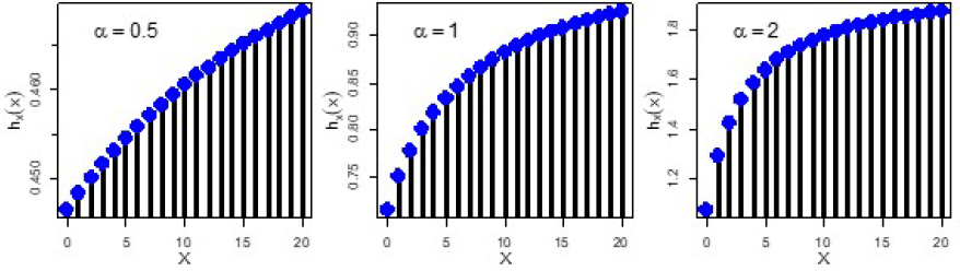
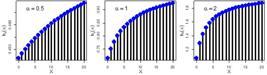
Since ξ ^′ (x) < 0, the h _x (x) of PFJD is increasing. Figure 3 shows the failure rate charts for a few different parameter values. It is clear that the rate shows a rising trend as the parameter value increase.

Figure 3
Shapes of Hazard function for varied values of parameter.

3 MATHEMATICAL PROPERTIES

In this section, we shall extract some important statistical properties of PFJD. Among them are moments and related measurements, generating functions, actuarial measures, and others.

3.1 Moments and Associated Measures

We present a model that has some statistical qualities that can be described using Raw and Central moments. Thus, we will start by calculating the factorial moments. One can compute the rth factorial moment of PFJD as

$$\begin{gathered} {\mu }_{\left(r\right)}\text{'}=E\left[E\right(X^{\left(r\right)}\left|\lambda \right]\text{Where}{X}^{\left(r\right)}=X(X-1)(X-2)\dots (X-r+1) \\ {\mu }_{\left(r\right)}\text{'}=\frac{\alpha }{2+{\alpha }^2}{\int }_0^{\infty }\left[\sum _{x=0}^{\infty }{x}^{\left(r\right)}\frac{e^{-\lambda }{\lambda }^x}{x!}\right]({\alpha }^3\lambda +2)e^{-\alpha \lambda }d\lambda , \end{gathered}$$

After some computations, we will obtain an expression for the r th factorial moment of PFJD as follows

${\mu }_{\left(r\right)}\text{'}=\frac{r![2+{\alpha }^2(r+1)]}{(2+{\alpha }^2){\alpha }^r}.$ (4)

The first four factorial moments can be obtained by substituting r = 1, 2, 3, and 4 in Eq. (4). The first four raw moments of PFJD can be attained by utilizing the association between factorial moments and raw moments. The mean, variance, and other important moment-associated measures are expressed as follows

$$\begin{gathered} \mathit{\text{Mean}}=\mu =\frac{2+2{\alpha }^2}{\alpha (2+{\alpha }^2)}. \\ \mathit{\text{Variance}}={\sigma }^2=\frac{2(2+2\alpha +4{\alpha }^2+3{\alpha }^3+{\alpha }^4+{\alpha }^5)}{{\alpha }^2(2+{\alpha }^2{)}^2}=\frac{2(2+4{\alpha }^3+{\alpha }^4)}{{\alpha }^2(2+{\alpha }^2{)}^2}+\mathit{\text{Mean}}. \\ \mathit{\text{Dispersion Index (DI)}}=\frac{2+2\alpha +4{\alpha }^2+3{\alpha }^3+{\alpha }^4+{\alpha }^5}{2\alpha +3{\alpha }^3+{\alpha }^5}. \\ \mathit{\text{Coefficient of Skewness (CoS)}}=\frac{8+12\alpha +28{\alpha }^2+30{\alpha }^3+20{\alpha }^4+18{\alpha }^5+7{\alpha }^6+3{\alpha }^7+{\alpha }^8}{\sqrt{2}(2+2\alpha +4{\alpha }^2+3{\alpha }^3+{\alpha }^4+{\alpha }^5{)}^{3/2}}. \\ \mathit{\text{Coefficient of Kurtosis (CoK)}}=\frac{72+144\alpha +368{\alpha }^2+512{\alpha }^3+504{\alpha }^4+500{\alpha }^5+328{\alpha }^6 \\ +198{\alpha }^7+104{\alpha }^8+31{\alpha }^9+13{\alpha }^{10}+{\alpha }^{11}}{2(2+2\alpha +4{\alpha }^2+3{\alpha }^3+{\alpha }^4+{\alpha }^5{)}^2}. \end{gathered}$$

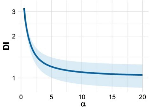
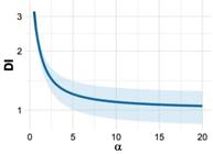
The moment-related metrics have been calculated for a range of model parameter values. Table 1 presents the findings. It is clear from these calculated figures that DI continues to be more than 1, indicating the occurrence of over-dispersion. Additionally, it is noted that the model is Leptokurtic in shape and has positive Skewness. The graphical presentation of DI is provided in Figure 4.

Table 1
Mean, Variance, DI, CoS, and CoK for chosen parameter values.

α	0.2	0.4	0.6	0.8	1	2	4	8	16
µ	5.09	2.68	1.92	1.55	1.33	0.83	0.47	0.24	0.12
σ 2	31.06	9.82	5.48	3.78	2.88	1.30	0.59	0.27	0.13
DI	6.09	3.66	2.85	2.43	2.16	1.56	1.26	1.12	1.06
CoS	2.00	2.00	1.98	1.95	1.91	1.83	1.97	2.37	3.09
CoK	9.01	8.95	8.75	8.47	8.21	7.59	7.95	9.68	13.57

Figure 4
DI of PFJD.

3.2 Generating Functions

3.2.1 Probability generating function (PGF)

PGF is a useful tool for working with discrete random variables. Its primary benefit is that it simplifies the process of describing the distribution of X+Y in the case where they are independent. It is possible to obtain the probability generating function of PFJD as

$$\begin{gathered} P_x\left(t\right)=\frac{\alpha }{(2+{\alpha }^2)(1+\alpha {)}^2}\left[{\alpha }^3{\sum _{x=0}^{\infty }(x+1)\left(\frac{t}{1+\alpha }\right)}^x+2(1+\alpha )\sum _{x=0}^{\infty }{\left(\frac{t}{1+\alpha }\right)}^x\right] \\ {P}_x\left(t\right)=\frac{\alpha }{(2+{\alpha }^2)(1+\alpha {)}^2}\left[\frac{{\alpha }^3(1+\alpha {)}^2}{(1+\alpha -t{)}^2}+\frac{2(1+\alpha {)}^2}{(1+\alpha -t)}\right] \end{gathered}$$

$P_x\left(t\right)=\frac{\alpha (2-2t+2\alpha +{\alpha }^3)}{(2+{\alpha }^2)(1+\alpha -t{)}^2}.$ (5)

3.2.2 Moment generating function (MGF)

Consider the MGF as an alternative method of displaying a random variable’s distribution. It can also be used to calculate the moments concerning origin, as suggested by the name itselffunction generating moments. If you take t= e ^t in Eq. (5), you will obtain the moment generating function of PFJD in the following way:

$M_x\left(t\right)=\frac{\alpha (2-2e^t+2\alpha +{\alpha }^3)}{(2+{\alpha }^2)(1+\alpha -e^t{)}^2}.$

3.3 Recurrence Relation of Probability

One can construct the recurrence relation for the probabilities of PFJD as

$\frac{P(x+1)}{P\left(x\right)}=\frac{\alpha }{2+{\alpha }^2}\left[\frac{{\alpha }^3(x+2)+2(1+\alpha )}{(1+\alpha {)}^{x+3}}\right]\times \frac{2+{\alpha }^2}{\alpha }\left[\frac{(1+\alpha {)}^{x+2}}{{\alpha }^3(x+1)+2(1+\alpha )}\right]$

$P(x+1)=\frac{2+2\alpha +(x+2){\alpha }^3}{(1+\alpha )[2+2\alpha +(x+1\left){\alpha }^3\right]}P\left(x\right).$ (6)

After obtaining P(0), we can easily calculate the various probabilitiesP(1), P(2), P(3),... using the relation given in above equation (6).

3.4 Actuarial Measures

Actuarial measures are the numerical instruments used in the field of actuarial sciences to evaluate financial risk, particularly in the insurance and pension industries. The actuaries find great use for these metrics when making decisions about capital management, pricing, and reserves [see; Bahnemann (2015)].

3.4.1 Mean Residual Life

The mean residual life, also known as the mean remaining lifetime (MRL), for a random variable X is the estimated remaining life X-t, given the item has survived to time i. Thus, stochastic aging and reliance for dependability can benefit greatly from the application of the MRL paradigm [see; Guess & Proschan (1988)]. For i=0, the distribution’s unconditional mean is a particular instance of MRL. The MRL is given as follows

$MRL=E(X-x|X\ge x)=\frac{1}{S_x\left(x\right)}\sum _{i=x+1}^{\infty }{S}_i\left(i\right),$

Here, x = 0, 1, 2, ...

If X is distributed as a PFJD, then its MRL is given by

$$\begin{gathered} MRL=\frac{(2+{\alpha }^2)(1+\alpha {)}^{x+2}}{2+2\alpha +{\alpha }^2+{\alpha }^3(x+2)}\sum _{i=x+1}^{\infty }\frac{2+2\alpha +{\alpha }^2+{\alpha }^3(i+2)}{(2+{\alpha }^2)(1+\alpha {)}^{i+2}} \\ MRL=\frac{2+2\alpha +{\alpha }^2+{\alpha }^3(x+3)}{\alpha [2+2\alpha +{\alpha }^2+(x+2\left){\alpha }^3\right]}. \end{gathered}$$

3.4.2 Value at Risk and Tail Value at Risk

A statistical metric called Value at Risk (VaR _p ) is used to estimate the possible decline in value of an asset or portfolio over a given holding time with a particular degree of confidence (say p). It is a widely used risk metric. Let X be the random variable for the loss. The PFJD’s VaR _p is calculated as

$P(X>{\eta }_p)=1-p,\text{and}{\eta }_p=F^{-1}\left(p\right),$

The value of p is the solution to equation; $\alpha \left[{\alpha }^3\right(x+2)+2(1+\alpha \left)\right]=(2+{\alpha }^2)(1+\alpha {)}^{x+2}(1-p)$. More precisely, we equate the CDF of PFJD to p and solve for p. And after considering a particular value of α and desired level of significance, we are able to PFJD’s VaR _p .

“Conditional tail expectation” or “tail conditional expectation” are other names for the Tail Value at Risk (TVaR _p ). It is a helpful statistic for figuring out the expected loss amount in the event that something happens with a lower likelihood than expected. A detailed version of these risk measures is provided by Hardy (2006). If X is a member of the PFJD, then X ^′ s TVaR _p is

$$\begin{gathered} TVa{r}_p=E\left(X\right|X>{\eta }_p)=\frac{1}{S_x\left({\eta }_p\right)}\sum _{i={\eta }_p}^{\infty }iP(X=x) \\ TVa{r}_p=\frac{(1+\alpha )[2+\alpha (1+{\eta }_p\left)\right(2+\alpha (2+\alpha (2+\alpha {\eta }_p\left)\right)\left)\right]}{\alpha [2+\alpha (2+\alpha +{\alpha }^2(2+{\eta }_p)\left)\right]}. \end{gathered}$$

The Table 2 lists some VaRp and T −VaRp measure values for PFJD for varied choices of the parameter value.

Table 2
Computed values of VARp and TVARp for four different values for the parameter with varied significance levels.

	α = 0.5	α = 1.0	α = 2	α = 3
Sig. Level	0.80	0.80	0.80	0.80
	0.85	0.85	0.85	0.85
	0.90	0.90	0.90	0.90
	0.95	0.95	0.95	0.95
	0.99	0.99	0.99	0.99
VaRp	3.3367	1.8889	1.0557	0.6698
	4.1060	2.3818	1.3845	0.9326
	5.1877	3.0687	1.8387	1.2949
	7.0305	4.2257	2.5959	1.8980
	11.2825	6.8507	4.2929	3.2471
T −VaRp	8.0368	5.5778	4.1057	3.3352
	9.1540	6.4690	4.9191	4.1412
	10.7279	7.7264	6.0795	5.3063
	13.4160	9.8767	8.0838	7.3466
	19.6457	14.8566	12.7707	12.1872

3.4.3 Expected Value Principle

A number of premium principles have been developed over time, and one of the most significant measures in the insurance and risk management fields is the expected value principle (EVP). These principles take into account the risk levels associated with different events when establishing insurance premiums. It specifies that the cost of insurance coverage, after accounting for risk loading, should be equal to the estimated value of the losses. We will now examine a risk loading parameter where τ ≥ 0. If (1 + τ) represents the factor of risk loading, then the EVP can be expressed mathematically as

$EVP(\tau ;.)=(1+\tau )E\left(X\right)=(1+\tau )\frac{2+2{\alpha }^2}{\alpha (2+{\alpha }^2)}.$

3.4.4 Exponential Premium Principle

The exponential premium principle (EPP) can be used to explain how, in the insurance and finance industries, premiums can increase considerably in direct proportion to risk factors or age. The EPP is very helpful in several insurance-related areas, including health, liability, and property insurance. It says that the likelihood of major loss events occurring rises quickly with increasing risk levels. The following is the general equation for EPP.

$\varphi (\epsilon -EPP(\tau ;.)=E(\epsilon -X),$

Here, ε denotes capital of a person, and ϕ(k) = −e ^−τk represents the function of exponential utility. As a result, the EPP comes out to be

$EPP(\tau ;.)=\frac{1}{\tau }{M}_X\left(t\right)=\frac{1}{\tau }\frac{\alpha (2-2e^t+2\alpha +{\alpha }^3)}{(2+{\alpha }^2)(1+\alpha -e^t{)}^2}.$

4 PARAMETRIC ESTIMATION

Two widely used techniques-the Bayesian estimation method and the method of maximum likelihood estimation-are used in this section to estimate the parameter of the PFJD model.

4.1 Method of Maximum Likelihood Estimation

The foundation for estimation is really simple. When sampling is done from a population that is represented by a particular distribution, knowing the parameter provides information about the entire population. The maximum likelihood approach is more frequently employed to determine the parameters of statistical models. Maximum likelihood estimation (MLE) is used to estimate the parameters of an assumed probability distribution based on observed data. Our goal in MLE is to maximize the probability of observing the data from the joint probability distribution given a probability distribution and its parameters.

If (x ₁ , x ₂ , . . . , x _n ) is independent and identically distributed random sample of size n from PFJD, then the log-likelihood function of PFJD can be defined as follows

$logL=n\log \alpha -n\log (2+{\alpha }^2)-n(\overline{x}+2)\log (1+\alpha )+\sum _{i=1}^n\log \left[{\alpha }^3\right(x_i+1)+2(1+\alpha \left)\right],$

Here, $\overline{x}$ is sample mean.

The maximum likelihood (ML) estimate of α is the solution to the following equation:

$\frac{d\log L}{d\alpha }=\frac{n}{\alpha }-\frac{2n\alpha }{2+{\alpha }^2}-\frac{n(\overline{x}+2)}{1+\alpha }+\sum _{i=1}^n\frac{3{\alpha }^2(x_i+1)+2}{{\alpha }^3(x_i+1)+2(1+\alpha )}=0,$

This cannot be solved analytically and thus calls for use of an appropriate numerical method. We have employed the optim command in R for this computation.

4.2 Bayesian Estimation

One alternative to the traditional MLE method is the Bayesian parameter estimation technique. For every unknown parameter in Bayesian estimation, a prior distribution needs to be defined. The Bayesian estimation for discrete distributions was studied extensively by Irony (1992). A detailed study pertaining to Bayesian Analysis of finite Poisson mixtures was provided by Dellaportas et al. (2011).

The likelihood function for the given set of data (x = x ₁ , x ₂ , ...x _n ) from a PFJD is given by

$L=\frac{{\alpha }^n}{(2+{\alpha }^2{)}^n(1+\alpha {)}^{2n+{\sum }_{i=1}^n{x}_i}}\prod _{i=1}^n\left[{\alpha }^3\right(x_i+1)+2(1+\alpha \left)\right].$

The posterior distribution function of the Bayesian model is produced by multiplying the prior distribution for the model parameter with the likelihood function for the given data using the Bayes theorem. The prior of α is denoted by p(α).

$p\left(\alpha \right|x)\propto L(\alpha \left|x\right)p\left(\alpha \right).$

An extensive research work related to the choice of prior distribution in case of Bayesian estimation was put forward by Seliem (2024). The gamma distribution is regarded as a prior distribution in our case with known hyper-parameters such α ∼ Gamma (a, b). The Gamma distribution is the conjugate prior for the Poisson and its compound distributions. This means the posterior distribution remains in the Gamma family, making Bayesian updating mathematically convenient. Further the Gamma distribution is highly flexible as it allows control over how much prior information influences inference. Furthermore the parameter of our model is non-negative; the Gamma distribution becomes a natural choice. Multiplying the likelihood by the prior yields the posterior expression, up to proportionality, and this can be expressed

$p\left(\alpha \right|x)\propto \frac{a^b}{\Gamma b}{e}^{-a\alpha }{\alpha }^{b-1}\frac{{\alpha }^n}{(2+{\alpha }^2{)}^n(1+\alpha {)}^{2n+{\sum }_{i=1}^n{x}_i}}\prod _{i=1}^n\left[{\alpha }^3\right(x_i+1)+2(1+\alpha \left)\right].$

Since the posterior density is not mathematically tractable, we will use the Markov Chain Monte Carlo (MCMC) method to simulate posterior samples in order to facilitate sample-based inference [see; Chib (2011)].

In this paper, we investigate how to simulate samples from the joint posterior distribution using MCMC methods that are implemented in the R program’s MCMCpack package. We produced 1006000 samples of the joint posterior distribution of interest for this reason. After 6000 simulated samples are burned in during the burn-in phase of the iterative process, the impacts of the original values are removed. In order to obtain roughly independent samples, a thinning interval of size 300 was employed. By calculating the expected value of the generated samples, the parameter Bayes estimates were obtained. The Geweke diagnostic test and Trace Plots were utilized to track the simulated sequences’ convergence. The Geweke convergence diagnostic is based on the asymptotic standard error of the difference divided by the difference between the two means of non-overlapping sections of a simulated Markov chain. If the equivalent absolute z score of a chain is less than 1.96, we can declare it to have found convergence because this z score asymptotically follows a normal distribution. Using the R software tool MCMCpack, the posterior summaries pertaining to our study were created.

It should be noted that our first selection of the hyper-parameters was subjective; we evaluated a number of settings and chose the ones that fit the data the best by calculating an appropriate statisticChi-square statistic, Kolmogorov-Smirnov (KS) statistic. Empirical Bayesian approaches frequently use this strategy, where the value of hyper-parameters is selected in order to improve model performance.

5 SIMULATION STUDY

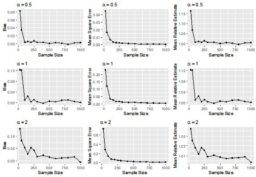
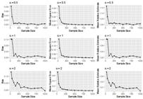
This part studies the estimating performance of the ML estimate using a thorough simulation exercise. Samples of different sizes are generated using PFJD, and three settings (α = 0.5, 1.0, and 2.0) are taken into consideration. The simulation process is based on one thousand iterations. Bias, Mean Square Error (MSE), and Mean Relative Estimate (MSE) values are provided by

$$\begin{gathered} Bias=\frac{1}{N}\sum _{i=1}^N({\hat{\alpha }}_i-\alpha ), \\ MSE=\frac{1}{N}\sum _{i=1}^N({\hat{\alpha }}_i-\alpha {)}^2, \\ MRE=\frac{1}{N}\sum _{i=1}^N\frac{{\hat{\alpha }}_i}{\alpha }. \end{gathered}$$

In Figure 5, the graphical view of the Bias, MSEs, and MREs is displayed. As sample size increases, the bias and MSEs for every choice of the parameter decrease. It is discovered that as the sample size grows, the MREs go closer to value one. As a result, we draw the conclusion that the MLE predicts the PFJD’s parameter effectively.

Figure 5
Bias, Mean Square Error, and Mean Relative Estimate for different parametric values.

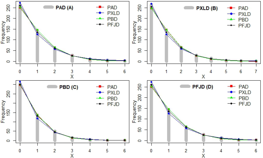
Remark 7. To showcase the enhanced flexibility of the PFJD compared to other Poisson mixture models discussed in existing literature, we conducted a second simulation process. For the estimation purpose, we made use of the maximum likelihood method of estimation. This experiment involved simulations based on various competing models with sample size of n=500 viz. Poisson-Ailamujia distribution (PAD), Poisson-XLindley distribution (PXLD), and PoissonBilal distribution (PBD). We set the initial parameter of all these models in such a manner that the generated data exhibited a declining pattern as the variable values increased. Table 3 presents the results of our simulation. This table provides comparison of true model parameter against predictable parameter (standard errors in parenthesis) across various compound probability models for a choice of compound probability models. Additionally, performance metrics including loglikelihood (L), AIC, BIC and Chi-square Goodness-of-fit (Chi-square value, degrees of freedom, and p value) are made available (Bold represents p-value > 0.05 & minimum loss under Information Criterions). Initially, when the data originated from PAD with parameter, β = 1.2 (Figure 6 (A)), we observed that the logarithm of the likelihood function for all the models is very close to one another, if not equal. When evaluating the Goodness-of-fit, it can be deduced that PFJD outperforms all other models with minimum chi-square value and highest p-value. Additionally, both AIC and BIC criteria suggest that our PFJD offers superior fitting.

Frm01 $\hat{\beta }$

Frm01 $\hat{\beta }$

Frm01 $\hat{\beta }$

Frm01 $\hat{\beta }$

Frm02 $\hat{\theta }$

Frm02 $\hat{\theta }$

Frm02 $\hat{\theta }$

Frm02 $\hat{\theta }$

Frm03 $\hat{\delta }$

Frm03 $\hat{\delta }$

Frm03 $\hat{\delta }$

Frm03 $\hat{\delta }$

Frm04 $\hat{\alpha }$

Frm04 $\hat{\alpha }$

Frm04 $\hat{\alpha }$

Frm04 $\hat{\alpha }$

Table 3
Outcome of generated data under PAD, PXLD, PBD, and PFJD.

Simulated Model	PAD	PXLD	PBD	PFJD
PAD (β= 1.2)	Frm01 = 1.2106(0.071)	Frm02 = 1.4155(0.079)	Frm03 =1.0092(0.059)	Frm04 =2.0168(0.166)
χ2	2.90, 4, 0.5736	1.54, 4, 0.8195	3.43, 4, 0.4874	0.32, 4, 0.9883
L	-628.5411	-628.3237	-628.3625	-627.1406
AIC	1259.0822	1258.6473	1258.7249	1256.2813
BIC	1263.2968	1262.8619	1262.9395	1260.4959
PXLD (θ = 1.3)	Frm01 = 1.1737(0.068)	Frm02 = 1.3793(0.077)	Frm03 =0.9786(0.057)	Frm04 =1.9136(0.159)
χ2	8.16, 4, 0.0858	2.70, 4, 0.6084	7.42, 4, 0.1153	3.45, 4, 0.4842
L	-641.1934	-638.6142	-640.9108	-638.5198
AIC	1284.3868	1279.2285	1283.8216	1279.0396
BIC	1288.6014	1283.4431	1288.0362	1283.2542
PBD (δ = 1.5)	Frm01 = 1.6949(0.112)	Frm02 = 1.8947(0.122)	Frm03 =1.4125(0.094)	Frm04 =3.0895(0.247)
χ2	1.64, 3, 0.6497	2.55, 3, 0.4649	1.43, 3, 0.6971	0.92, 3, 0.8205
L	-523.233	-524.1629	-523.1642	-522.8466
AIC	1048.466	1050.3258	1048.3285	1047.6933
BIC	1052.681	1054.5404	1052.5431	1051.9079
PFJD (α = 2.0)	Frm01 = 1.2077(0.070)	Frm02 = 1.4127(0.793)	Frm03 =1.0067(0.059)	Frm04 =2.0119(0.166)
χ2	5.78, 4, 0.2154	3.56, 4, 0.4677	5.53, 4, 0.2364	2.98, 4, 0.5601
L	-629.1947	-629.1224	-629.0052	-627.9061
AIC	1260.3894	1260.2449	1260.0103	1257.8121
BIC	1264.6040	1264.4595	1264.2250	1262.0267

Figure 6
Observed & Expected frequency plots under PAD (A), PXLD (B), PBD (C) and PFJD (D).

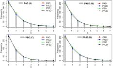
The second row of data in the table corresponds to simulated data generating using the PXLD with a parameter θ = 1.3 (see Figure 6 (B)). Similar to the previous case, it is observed that all the distributions fit this data at 5% level of significance, with PAD having the lowest p-value and PXLD having the highest p-value. Notably, the PFJD exhibits the lowest AIC and BIC values. This became evident when the AIC and BIC values of PFJD were put side by side to AIC and BIC values corresponding to other models.

In this scenario we simulated data using PBD with the specified parameter δ = 1.5 (see Figure 6 (C)), and our findings indicate that the PFJD demonstrated the best fit when considering various measures of performance. The final piece of this simulation method produces data from the PFJD, with a parameter value α = 2.0 (see Figure 6 (D)). The fitting results reveal that all the models accepted the null hypothesis, but it is noteworthy that the PFJD performed better than other competing models across all the examined metrics.

Considering everything that has occurred, it is evident that PFJD has demonstrated significant versatility in effectively modeling count data coming from different models which are overdispersed in nature.

6 DATA APPLICATIONS

We have used the COVID-19 deaths in China and Armenia as a means of evaluating the suitability of our suggested model. Furthermore, we juxtaposed the outcomes of our suggested model with those of alternative statistical models. The Poisson distribution (PD), Negative Binomial distribution (NBD), Poisson-Ailamujia distribution (PAD), Poisson-XLindley distribution (PXLD), and Poisson-Bilal distribution (PBD) are the models we took into consideration for comparison. We utilized the maximum likelihood estimation approach to estimate the parameters of each distribution. The Bayesian approach was also employed for our model. Data sets from the real world have been taken into account. We considered a few features of our data sets before data fitting. These consist of the Mean, Variance, and Dispersion Index.

6.1 Data Set 1 (COVID-19 Deaths in Armenia)

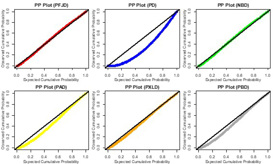
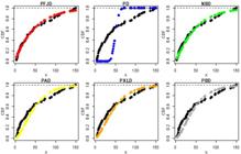
We start by using the dataset of newly reported COVID-19-related deaths in Armenia every day. As of January 10, 2021, the data can be obtained at https://www.worldometers.info/coronavirus/ country/armenia/. The daily fresh COVID cases for the period of February 15, 2020, to October 4, 2020 are contained in them. Using the specified statistical methods-log-likelihood (L), Akaike Information Criterion (AIC), Bayesian Information Criterion (BIC), Chi-square statistic, and pvalue-we compare the competing distributions to the PFJD. The dataset from Armenia has an empirical mean, variance, and DI of 4.193, 18.80, and 4.48 respectively. For this dataset, Table 4 contains the fitting findings. The dataset’s PP charts under PFJD and other rival models are shown in Figure 7. With the maximum p-value and the least amount of loss under the information criteria, it is clear from the fitting results that the PFJD provides better fitting to this data set.

Table 4
Data set 1.

Daily Covid -19 Cases	0	1	2	3	4	5	6	7	8	9	10	11	12	13	14	15	< 16
Frequency	56	31	22	25	11	14	14	10	11	3	10	7	4	5	2	2	6

Table 5
Results of model fitting for data set 1.

Model	MLEs(S.E)	χ 2	df	p-value	L	AIC	BIC
PFJD	0.24(0.02)	10.46	8	0.2342	-592.7889	1187.5778	1191.0289
PD	4.19(0.13)	485.49	7	<0.001	-827.4472	1656.8943	1660.3454
NBD	1.00(0.13)	10.47	7	0.1634	-592.7991	1189.5982	1196.5003
	0.19(0.02)
PAD	0.24(0.01)	64.65	8	<0.001	-612.7339	1227.4677	1230.9188
PXLD	0.37(0.02)	18.03	8	0.0210	-594.864	1191.7280	1195.1790
PBD	0.20(0.01)	57.74	8	<0.001	-611.8097	1225.6193	1229.0704

Figure 7
PP plots for data set 1 under different considered models.

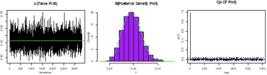
In Bayesian data analysis, it was assumed that the parameter α of the PFJD had an approximate gamma distribution, i.e., α ∼ Gamma (0.01, 0.001). The posterior samples for the parameter α are provided in the Figure 8. ACF plot, Posterior Density, and Trace plot are used to evaluate the MCMC draws across several iterations. It’s fascinating to see from the Trace plot that the samples generated reached a satisfactory level of convergence. The posterior samples don’t seem to be connected, according to the ACF plot. Furthermore, the samples have sufficiently converged to a stable distribution, as indicated by the Geweke test’s z-score of -0.09069, which is less than 1.96. With a standard deviation of 0.01904283, we have a posterior mean for α as α _Bayes = 0.2462148, and the corresponding 95% maximum density interval is (0.2111678, 0.2848102). Furthermore, the value of Chi-square is 10.46 with a p-value of 0.2342 indicating the Bayes estimator provides similar sort of fitting results as that of the ML estimator.

Figure 8
Trace plot, Posterior density, and ACF plots constructed on data set 1.

6.2 Data Set 2 (COVID-19 Deaths in China)

COVID-19 claimed a number of lives in China between January 23, 2020, and March 28, 2020. The information on daily deaths due to COVID-19 in China during this period are the following: 8, 16, 15, 24, 26, 26, 38, 43, 46, 45, 57, 64, 65, 73, 73, 86, 89, 97, 108, 97, 146, 121, 143, 142, 105, 98, 136, 114, 118, 109, 97, 150, 71, 52, 29, 44, 47, 35, 42, 31, 38, 31, 30, 28, 27, 22, 17, 22, 11, 7, 13, 10, 14, 13, 11, 8, 3, 7, 6, 9, 7, 4, 6, 5, 3, and 5. For this dataset, some descriptive metrics (mean, variance, and dispersion index) are 47.74, 1924.84, and 38.70. The dataset is accessible at https://www.worldometers.info/country/china/coronavirus/. For the second dataset, we obtain the model selection metrics (KS, AIC, and BIC) and the ML estimates for the parameter. The fitting results for this dataset are itself present in Table 6. The expected and observed CDF of this dataset under PFJD and other competing models is provided in the Figure 9. From the fitting results, it is very obvious from different performance metrics that the PFJD is providing better fitting to this data set as compared to other models.

Table 6
Fitting results of dataset 2.

Model	MLEs(S.E)	K-S Value	p-value	L	AIC	BIC
PFJD	0.0201 (0.0025)	0.0853	0.7227	-324.5117	651.0234	653.2130
PD	49.7424 (0.8681)	0.4975	<0.001	-1409.782	2821.565	2823.754
NBD	1.1815 (0.1910)	0.0936	0.6089	-324.0081	652.0162	656.3955
	0.0232 (0.0044)
PAD	0.0200 (0.0017)	0.1672	0.0499	-329.9865	661.9731	664.1627
PXLD	0.0387 (0.0034)	0.1516	0.0963	-328.3757	658.7514	660.9410
PBD	0.0168 (0.0015)	0.1618	0.0631	-329.5817	661.1634	663.3531

Figure 9
Observed and Expected CDF for data set 2 under various models.

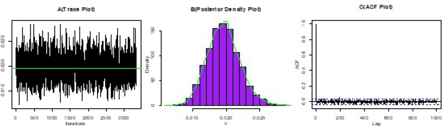
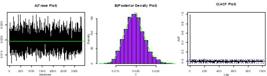
In Bayesian data analysis, it was assumed that the parameter α of the PFJD had an approximate gamma distribution, i.e., α ∼ Gamma (0.1, 100). The posterior samples for the parameter α are shown in Figure 10. ACF plot, Posterior Density, and Trace plot are used to evaluate the MCMC draws across several iterations. It’s fascinating to see from the Trace plot that the samples generated attain a satisfactory level of convergence as evidenced by the stable and consistent fluctuations around a constant mean. The posterior samples don’t seem to be connected, according to the ACF plot. Furthermore, the samples have sufficiently converged to a stable distribution, as indicated by the Geweke test’s z-score of 0.03029, which is less than 1.96. With a standard deviation of 0.002387031, we have a posterior mean for α as α _Bayes = 0.01954747, and the corresponding 95% maximum density interval is (0.01519000, 0.02466028). Furthermore, the value of KS statistic is 0.0772 with a p-value of 0.8261 indicating the Bayes estimator provides better fitting results than the ML estimator.

Figure 10
Trace plot, Posterior density, and ACF plots constructed on data set 2.

The fitting performance of both the data sets clearly shows that our suggested model, PFJD, performs better than other models that have been taken into consideration as evident from various performance metrics. It is worth mentioning that it made sense to use KS test statistic in case of the second data set because it works with cumulative distributions and doesn’t require binning, especially since this very data set wasn’t well-binned. Further, in the rest of the analysis, we relied on the Chi-square statistic as the data was categorised and allows comparison between observed and expected frequencies within defined intervals.

7 COUNT DATA REGRESSION

This section presents the PFJ regression model, a novel count data regression approach based on the PFJD. The basics of count data regression can be found in the research of Cameron & Trivedi (2013).

7.1 PFJ Regression Model

With a random variable Y ~ PFJD, the PMF of the PFJD may be expressed in terms of mean, E(Y ) = µ > 0, and can be obtained by applying the re-parameterization as expressed below

$\alpha =\frac{4-6{\mu }^2+2{\left(8+9{\mu }^2+3\sqrt{3}\sqrt{{\mu }^2(16-13{\mu }^2+8{\mu }^4)}\right)}^{1/3}+{\left(8+9{\mu }^2+3\sqrt{3}\sqrt{{\mu }^2(16-13{\mu }^2+8{\mu }^4)}\right)}^{2/3}}{3\mu {\left(8+9{\mu }^2+3\sqrt{3}\sqrt{{\mu }^2(16-13{\mu }^2+8{\mu }^4)}\right)}^{1/3}}$

Let us assume that $[8+9{\mu }^2+3\sqrt{3}\sqrt{{\mu }^2(16-13{\mu }^2+8{\mu }^4)}]=m$

The PMF after applying the re-parameterization comes out to be

$$\begin{gathered} P(Y=y|\mu )=\frac{\frac{2+(4-6{\mu }^2)m^{-1/3}+m^{1/3}}{3\mu }}{2+{\left(\frac{2+(4-6{\mu }^2)m^{-1/3}+m^{1/3}}{3\mu }\right)}^2} \\ \times \left[\frac{{\left(\frac{2+(4-6{\mu }^2)m^{-1/3}+m^{1/3}}{3\mu }\right)}^3(y+1)+2\left(1+\frac{2+(4-6{\mu }^2)m^{-1/3}+m^{1/3}}{3\mu }\right)}{{\left(1+\frac{2+(4-6{\mu }^2)m^{-1/3}+m^{1/3}}{3\mu }\right)}^{y+2}}\right] \end{gathered}$$

This formula establishes the PMF of a distribution represented by PFJ(µ), meaning that Y ∼ PFJ(µ). If the response variable fulfils Y _i ∼ PFJ(µ _i ), the i ^th mean of response variable is connected to the covariates via the log-link function provided by

${\mu }_i=\exp \left({x_i}^T\beta \right);i=1,2,3,...,n$

Here, β = (β ₀ , β ₁ , β ₂ , ...β _p ) represents the regression coefficients vector and $x_i^T=\left(x_{i1},x_{i2},...x_{ip}\right)$ is the covariates vector.

Adding the log-link yields the log-likelihood function of the PFJ regression model, which is given by

$\log L\left(\Theta \right)=\sum _{i=1}^n\left\{\begin{array}{c}\log [2+(4-6{{\mu }_i}^2)m^{-1/3}+m^{1/3}]-2\log [6{\mu }_i+2+(4-6{{\mu }_i}^2)m^{-1/3}+m^{1/3}]\\ +\log \left\{\right(y_i+1\left)\right[2+(4-6{{\mu }_i}^2)m^{-1/3}+m^{1/3}]\\ +18{{\mu }_i}^2[3{\mu }_i+2+(4-6{{\mu }_i}^2)m^{-1/3}+m^{1/3}]\}\\ -(y_i+2)\log [3{\mu }_i+2+(4-6{{\mu }_i}^2)m^{-1/3}+m^{1/3}]\\ +(y_i+3)\log 3+(y_i+3)\log {\mu }_i\end{array}\right\}$

Here, Θ = c(β) represents the set of parameters that are determined by using the R software’s optim function to maximize log-likelihood function.

7.2 Application of PFJ Regression Model

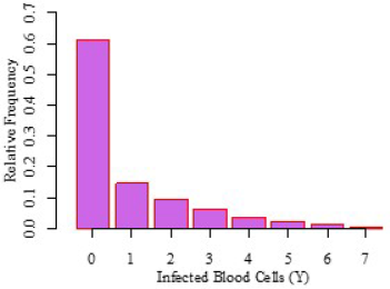
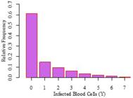
We take into account the data set that Ligges & Crawley (2007) reported. The information shows the number of infected blood cells (per millimetre squared) on microscope slides. 511 people in total who were chosen at random were taken into consideration. The goal of this study is to ascertain how the response variable, ”number of infected blood cells (Y) reported,” is affected by covariates such as an individual’s age, weight, sex, and smoking status. The bar plot showing the quantity of contaminated blood cells is shown in Figure 11.

Table 7
Covariates Description.

Covariates	Explanation
Sex	1-male ; 0-female
Smoking	1-smoker ; 0-otherwise
Young	1-young age ; 0-otherwise
Mid-Age	1-mid age ; 0-otherwise
Over-Weight	1-over weight ; 0-otherwise
Obese	1-obese ; 0-otherwise

Figure 11
The response variable’s bar plot.

Using the following log-link function, the covariates are associated with the i ^th response mean.

$\log \left({\mu }_i\right)={\beta }_0+{\beta }_{1}Sex+{\beta }_{2}Smoking+{\beta }_{3}Young+{\beta }_{4}MidAge+{\beta }_{5}OverWeight+{\beta }_{6}Obese.$

Poisson regression and the suggested regression model are used to fit the data. Both regression models indicate that the variables, sex and age (young and mid age), are statistically nonsignificant for modeling the response variable based on the fitting findings shown in Table 8; as a result, they are eliminated from further discussion. The fitted regression models’ performance is assessed using the widely-used model criteria of minus log-likelihood, AIC, and BIC. Table 8 shows that the PFJ regression model has lower AIC and BIC values than the Poisson regression, indicating that it fits better than the Poisson regression model. It should be noted that the model with the lowest AIC and BIC values is thought to fit better.

Table 8
The regression analysis of the quantity of blood cells infected.

Covariates	Poisson Regression					PFJ Regression
	Est.	S.E.	z-value	p-value	CI (95%)	Est.	S.E.	z-value	p-value	CI (95%)
Intercept	-1.173	0.12	-9.49	<0.001	(-1.42;-0.94)	-1.113	0.15	-7.01	<0.001	(-1.42;-0.80)
Sex	0.124	0.10	1.13	0.256	(-0.09;0.34)	0.204	0.15	1.36	0.173	(-0.09;0.50)
Smoking	1.305	0.11	11.70	<0.001	(1.09;1.53)	1.090	0.15	6.98	<0.001	(0.78;1.40)
Young	-0.059	0.12	-0.47	0.634	(-0.30;0.18)	0.042	0.18	0.23	0.818	(-0.32;0.40)
Mid-Age	-0.055	0.12	-0.44	0.658	(-0.30;0.19)	-0.037	0.18	-0.20	0.837	(-0.39;0.32)
Overweight	0.531	0.13	4.08	<0.001	(0.28;0.79)	0.512	0.17	2.88	<0.001	(0.16;0.86)
Obese	0.925	0.11	7.86	<0.001	(0.70;1.16)	0.848	0.16	5.09	<0.001	(0.52;1.17)
l	658.6965					625.1325
AIC	1331.393					1262.265
BIC	1361.048					1287.683

Consequently, the fitted model can be described as follows using the PFJ regression model:

$\log \left({\hat{\mu }}_i\right)=-1.113+1.090\mathit{\text{Smoking}}+0.512\mathit{\text{OverWeight}}+0.848\mathit{\text{Obese}}.$

Furthermore, it appears from the fitted PFJ regression model that smoking and being overweight or obese both increase the quantity of infected blood cells (per mm ² ).

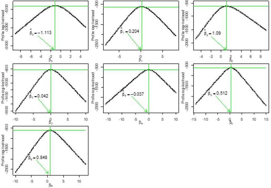
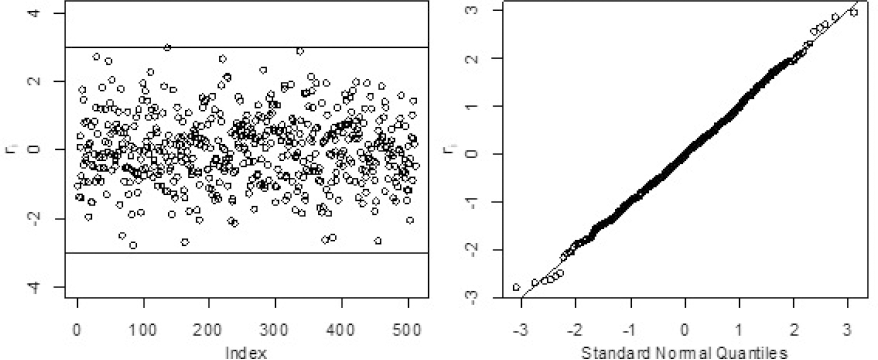
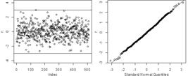
In order to verify the underlying assumptions of the model and ensure that it is adequate, residuals are essential. When working with discrete response variables, randomized quantile residuals are thought to be more suitable than other residuals like Pearson and deviance residuals for examining the suitability of the model and underlying assumptions [see; Dunn & Smyth (1996)]. The profile log-likelihood plots for the PFJ regression model’s parameters are displayed in Figure 12. Each of these plots demonstrates that the parameter estimates correspond to the real maxima’s of the log-likelihood function. Figure 13 shows randomized quantile residuals and the normal QQ-plots respectively. It is clear that no observation can be regarded as a potential outlier. Additionally, the normality is depicted by the QQ-plots of the randomized quantile residuals, and the Shapiro-Wilk test (p-value = 0.7739) supports this. Based on all of these findings, we deduce that our model fits the data quite well.

Figure 12
The log-likelihood profile graphs of the PFJ regression model for the cells data set.

Figure 13
The randomized quantile residuals and the normal Q-Q plot for cells data set.

8 CONCLUSION

Finding probability models that can handle over-dispersed data is crucial in the context of over-dispersion in order to select the appropriate models for various scenarios that yield better matches. In light of this, we studied a unique probability model and the related count data regression model. Poisson mixture modeling has been taken into consideration in the study of this innovative model. The model’s several statistical measures have specific expressions that have been derived. Additionally, actuarial measures have been thoroughly examined. Maximum likelihood method and Bayesian technique of estimation was utilized for the estimation and a thorough simulation was run to assess the validity of ML estimates and the suitability of the PFJ model with data simulated from competing models. The Bayesian estimation was carried out using the MCMC method as the expressions were not in the closed form. Two distinct data sets that represented the COVID-19 deaths were fitted with the distribution. The PFJ model was found to fit more closely than competing models based on the model comparison criteria. Additionally, a novel regression model was created and fitted to a dataset that showed the quantity of contaminated blood cells. The outcomes were then contrasted with the Poisson regression fitting results. The PFJ model was found to suit the data well based on the performance measures. Additionally, randomized quantile residuals were employed for the fitted regression model’s residual analysis, which once again verified the validity of the model. We believe that the PFJ model will gain traction and find broad use in the analysis of real-world count data sets from a variety of domains, given its attributes and fitting outcomes.

Acknowledgements

We would like to thank the Editor-in-chief and anonymous referees for their comments which we believe have enhanced the quality of this paper. The first author is particularly thankful to the Department of Science and Technology (Government of India) for INSPIRE fellowship (DST/INSPIRE/03/2022/002460).

References

• AHMAD PB & WANI MK. 2023. A New Compound Distribution and Its Applications in Overdispersed Count Data. Annals of Data Science, Available at: https://doi.org/10.1007/s40745-02300478-0
  » https://doi.org/10.1007/s40745-02300478-0
• ALTUN E. 2020. A new one-parameter discrete distribution with associated regression and integer-valued autoregressive models. Mathematica Slovaca, 70(4): 979-994. Available at: https://doi.org/10.1515/ms-2017-0407
  » https://doi.org/10.1515/ms-2017-0407
• BAGNOLI M & BERGSTROM T. 2005. Log-concave probability and its applications. Economic Theory, 26(2): 445-469. Available at: https://doi.org/10.1007/s00199-004-0514-4
  » https://doi.org/10.1007/s00199-004-0514-4
• BAHNEMANN D. 2015. Distributions for actuaries. CAS monograph series, 2: 1-200.
• BAKOUCH HS, JAZI MA & NADARAJAH S. 2012. A new discrete distribution. Statistics, 48(1): 200-240. Available at: https://doi.org/10.1080/02331888.2012.716677
  » https://doi.org/10.1080/02331888.2012.716677
• CAMERON AC & TRIVEDI PK. 2013. Regression analysis of count data. No. 53). Cambridge university press.
• CHIB S. 2011. Introduction to Simulation and MCMC Methods. In: The Oxford Handbook of Bayesian Econometrics. pp. 182-217. Available at: https://doi.org/10.1093/oxfordhb/9780199559084.013.0006
  » https://doi.org/10.1093/oxfordhb/9780199559084.013.0006
• DELLAPORTAS P, KARLIS D & XEKALAKI E. 2011. Bayesian Analysis of Finite Poisson Mixtures.
• DUNN PK & SMYTH GK. 1996. Randomized quantile residuals. Journal of Computational and graphical statistics, 5(3): 236-244.
• EKEMEZIE DFN & OBULEZI OJ. 2024. The Fav-Jerry Distribution: Another Member in the Lindley Class with Applications. Earthline Journal of Chemical Sciences, 793-816. Available at: https://doi.org/10.34198/ejms.14424.793816
  » https://doi.org/10.34198/ejms.14424.793816
• GOFFARD PO, JAMMALAMADAKA SR & MEINTANIS SG. 2022. Goodness-of-Fit Procedures for Compound Distributions with an Application to Insurance. Journal of Statistical Theory and Practice, 16(3). Available at: https://doi.org/10.1007/s42519-022-00276-6
  » https://doi.org/10.1007/s42519-022-00276-6
• GREENWOOD M & YULE GU. 1920. An Inquiry into the Nature of Frequency Distributions Representattive of Multiple Happenings with Particular Reference to the Occurrence of Multiple Attacks of Disease or of Repeated Accidents. Journal of the Royal Statistical Society, 83(2): 255. Available at: https://doi.org/10.2307/2341080
  » https://doi.org/10.2307/2341080
• GUESS F & PROSCHAN F. 1988. 12 Mean residual life: Theory and applications. Quality Control and Reliability, pp. 215-224. Available at: https://doi.org/10.1016/s0169-7161(88)07014-2
  » https://doi.org/10.1016/s0169-7161(88)07014-2
• HARDY MR. 2006. An introduction to risk measures for actuarial applications. SOA syllabus study note, 19.
• HASSAN A, SHALBAF GA, BILAL S & RASHID A. 2020. A New Flexible Discrete Distribution with Applications to Count Data. Journal of Statistical Theory and Applications, Available at: https://doi.org/10.2991/jsta.d.200224.006
  » https://doi.org/10.2991/jsta.d.200224.006
• IRONY TZ. 1992. Bayesian estimation for discrete distributions. Journal of Applied Statistics, 19(4): 533-549. Available at: https://doi.org/10.1080/02664769200000049
  » https://doi.org/10.1080/02664769200000049
• IRSHAD MR, SREE A & MAYA R. 2024. The Poisson Fav-Jerry distribution and its Inference properties. Available at: https://www.researchgate.net/publication/381429113
  » https://www.researchgate.net/publication/381429113
• KEILSON J & GERBER H. 1971. Some Results for Discrete Unimodality. Journal of the American Statistical Association, 66(334): 386-389. Available at: https://doi.org/10.1080/01621459.1971.10482273
  » https://doi.org/10.1080/01621459.1971.10482273
• LIGGES U & CRAWLEY MJ. 2007. The R Book. Stat Papers, 50: 445-446. Available at: https://doi.org/10.1007/s00362-008-0118-3
  » https://doi.org/10.1007/s00362-008-0118-3
• SANKARAN M. 1970. Note: The Discrete Poisson-Lindley Distribution. Biometrics, 26(1): 275. Available at: https://doi.org/10.2307/2529053
  » https://doi.org/10.2307/2529053
• SEGHIER FZ & ZEGHDOUDI H. 2021. A Poisson XLindley Distribution with Applications. Available at: https://doi.org/10.21203/rs.3.rs-343104/v1
  » https://doi.org/10.21203/rs.3.rs-343104/v1
• SELIEM MM, KAMEL AR, TAHA IM & EL-NASR ABU MM. 2024. A Note on Prior Selection in Bayesian Estimation. Statistics, Optimization & Information Computing, 13(2): 795-806. Available at: https://doi.org/10.19139/soic-2310-5070-1752
  » https://doi.org/10.19139/soic-2310-5070-1752
• SHANKER R. 2016. On Poisson-Akash Distribution and its Applications. Biometrics & Biostatistics International Journal, 3(5). Available at: https://doi.org/10.15406/bbij.2016.03.00075
  » https://doi.org/10.15406/bbij.2016.03.00075
• TAHIR MH & CORDEIRO GM. 2016. Compounding of distribution: a survey and new generalized classes. Journal of Statistical Distributions and Applications, 3(1). Available at: https://doi.org/10.1186/s40488-016-0052-1
  » https://doi.org/10.1186/s40488-016-0052-1
• WANI MK & AHMAD PB. 2023. Zero-inflated Poisson-Akash distribution for count data with excessive zeros. Journal of the Korean Statistical Society, Available at: https://doi.org/10.1007/s42952-023-00216-5
  » https://doi.org/10.1007/s42952-023-00216-5
• XEKALAKI E. 2014. On the distribution theory of over-dispersion. Journal of Statistical Distributions and Applications , 1(1). Available at: https://doi.org/10.1186/s40488-014-0019-z
  » https://doi.org/10.1186/s40488-014-0019-z
• ZAMANI. 2010. Negative Binomial-Lindley Distribution and Its Application. Journal of Mathematics and Statistics, 6(1): 4-9. Available at: https://doi.org/10.3844/jmssp.2010.4.9
  » https://doi.org/10.3844/jmssp.2010.4.9

• Funding
  The study received no external funding.
• Data Availability
  All the used data is provided within the manuscript either as an external link or reference.
• Ethical Statement
  As such, we affirm that the manuscript at hand is wholly our work. It should be noted that, except from the mentioned citations, this manuscript does not include any previously published results.

Edited by

• Editor responsible for the review
  Editor-in-Chief: Annibal Parracho Sant’Anna.

Data availability

All the used data is provided within the manuscript either as an external link or reference.

Publication Dates

• Publication in this collection
  04 July 2025
• Date of issue
  2025

History

• Received
  20 Jan 2025
• Accepted
  20 Apr 2025