Influence of stratigraphic variability on 2D and 3D factors of safety: a numerical investigation of tailings dam embankments

Abstract

Past research has focused on spatial variability or the influence of randomly distributed strength on slope stability. This research explores stratigraphic variability, specifically the influence of positional changes in the boundary between two materials of very different strengths on stability. Specifically, the boundary between drained and undrained material commonly present in upstream tailings dams. Two-dimensional (2D) and three-dimensional (3D) slope stability analyses are compared. The study showed that when a single random 2D cross-section was selected, this had an 11% probability of being unsafe (i.e., the resulting 2D factor of safety was higher than the 3D factor of safety calculated considering stratigraphic variability), while extrapolating a randomly selected 2D section to represent the entire 3D slope (i.e., ignoring stratigraphic variability) increased this risk to 46%. The reason why an extrapolated 3D slope stability analysis was unconservative is that, in many instances it failed to account for weak sides, toe, and back scarp conditions that existed when stratigraphic variability along the length of the slope was taken into consideration. These features can be overlooked when an analysis assumes homogeneity and highlights the importance of investigating conditions along the length of a slope particularly if a 3D analysis is to be performed.

Keywords:
Slope stability; Stratigraphic variability; Two-dimensional; Three-dimensional; Tailings dam

1. Introduction

Random field theory has been used by various authors to investigate the influence of soil variability on slope stability (Hicks et al., 2008; Hicks & Spencer, 2010; Li et al., 2013; Varkey et al., 2017, 2018; Hicks & Li, 2018; Liu et al., 2018; Zhang et al., 2022; Wu et al., 2024). However, the forensic analysis of failures suggests that slope stability is often controlled by specific stratigraphic layers or phreatic conditions rather than random variability (Duncan et al., 2014). This calls into question conclusions drawn from studies in which strength parameters are randomly distributed. While parameters will vary within a stratigraphic layer, variability in the boundary between stratigraphic layers is likely of greater consequence to stability. This stratigraphic variability has received much less attention, and studies are typically restricted to varying parameters within layered systems (Lim et al., 2015a, b).

A widely stated view in the literature is that two-dimensional (2D) slope stability analysis yields a lower factor of safety (F) compared to three-dimensional (3D) analyses (Albataineh, 2006; Griffiths & Marquez, 2007; Michalowski, 2010; Lim et al., 2015a, b; Chakraborty & Goswami, 2016; Chaudhary et al., 2016). This is primarily attributed to 2D methods assuming plane strain conditions, which neglect the stabilizing effects of side resistance or end confinement considered to be present in 3D failures. However, the stabilizing effects of side resistance are questioned particularly as the Kettleman Hills landfill failure showed that 3D F were approximately 10-15% lower than those based on 2D analyses of representative cross-sections (Seed et al., 1990). Relying on 3D effects to demonstrate that the factor of safety is adequate is therefore not considered wise, as the safety of the situation is likely marginal (Fell et al., 2015).

Studies using random field theory provide useful insights to understand how variability impacts the difference between 2D and 3D factors of safety. Work by Hicks et al. (2008) and Hicks & Spencer (2010) showed that the scale of fluctuation results in distinct failure modes. For low fluctuations, failures tend to be continuous over the entire length of the slope, but for high fluctuations failures tend to be layered. Between these two extremes failures tended to be more distinct and align more closely with observed behavior. Li et al. (2013) showed that these conclusions are influenced by model complexity for high fluctuations. Hicks & Li (2018) showed that 3D analyses generally result in lower F compared to the 2D analyses. This was because 2D models often overestimate F by failing to capture localized and variable failure paths. Varkey et al. (2017, 2018) further showed that cross-correlation between shear strength parameters significantly influences reliability with negative correlation increasing stability and positive correlation reducing it.

Lim et al. (2015a) contributed a complementary perspective by focusing on the stability of two-layered undrained clay slopes using finite element upper and lower bound limit analysis methods. The study highlighted the significant influence of 3D boundary effects, particularly the slope’s length-to-height ratio (L/H), on failure mechanisms. As L/H increases, the stability number rises, indicating greater risk, especially when the strength contrast between layers is high. The research identified that steep slopes tend to exhibit toe failure modes, while gentler slopes showed a mix of toe and base failures depending on the strength ratio. These findings reinforce the importance of 3D modeling in capturing the nuanced behavior of stratified soils and align with earlier work recognizing the limitations of simplified 2D approaches.

Studies by Zhang et al. (2022), Wu et al. (2024) and Liu et al. (2018) showed that 2D analyses, while computationally efficient, often overestimate F and sliding volumes, leading to conservative or misleading designs. In contrast, 3D analyses capture more realistic failure mechanisms, including multiple localized failures along the slope, which 2D models often miss. Zhang et al. (2022) noted that failure probabilities are generally lower in 3D, especially for longer slopes and larger fluctuation scales. Wu et al. (2024) confirmed that 3D models offer broader failure characteristics and more accurate reliability assessments. Liu et al. (2018) proposed a practical compromise by identifying the most pessimistic cross-section for 2D analysis, offering a conservative yet efficient alternative. Collectively, these studies support the use of 3D modeling in spatially variable soils.

As noted earlier, failures often stem from stratigraphic, rather than random, variability. Stratigraphic variability arises predominantly from geomorphological processes and therefore needs to be investigated within a geomorphological context. This study therefore examined the stratigraphic variability that arises from subaerial deposition of tailings (i.e., deposited in air), which causes coarse material to settle near the dam’s perimeter and fine material to accumulate in the center. The outer zone typically desaturates and strengthens, whereas the inner zone remains wet and weak (Donaldson, 1960; MacRobert & Blight, 2013). This natural process is used to construct upstream tailings dams and can result in a variable boundary between strong, dilative tailings (in the desaturated zone) and weak, contractive material in the inner zone. The extent of the desaturated zone varies with each deposition and results in a varying stepped stratigraphy around the perimeter of the dam. This study aims to quantify how this stratigraphic variability influences the factor of safety outcomes in the 2D and 3D analysis of upstream tailings dams. Stratigraphic variability likely has a significant impact on 3D slope stability analysis and requires investigation as 3D methods become more widely adopted.

2. Investigation approach

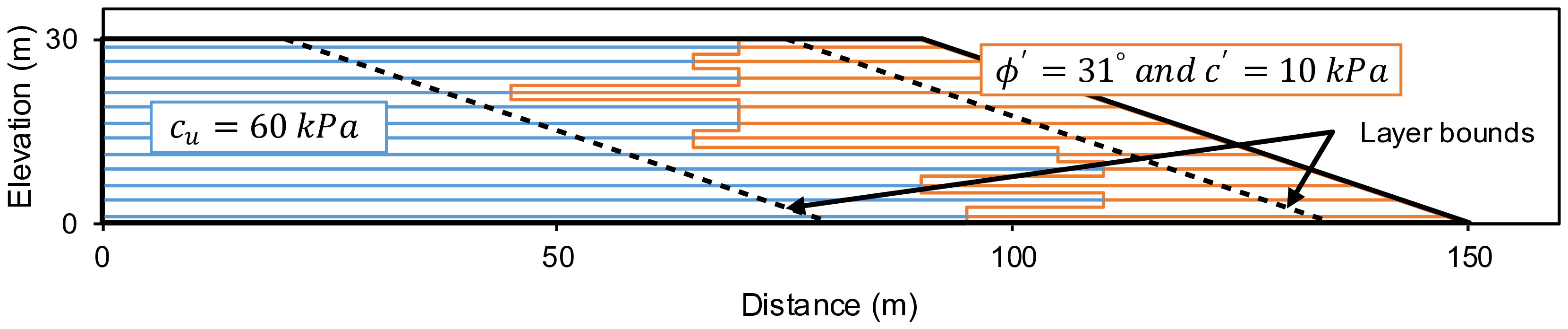
The geometry and number of scenarios used to investigate stratigraphic variability were limited by software constraints in analyzing highly stepped geometries and by the time required to build 2D and 3D geometries. The outer cross-sectional geometry had a constant height of 30 m, with a 1V:2H slope, and a base width of 150 m, which is considered typical for many tailings dams. The variable boundary between dilative and contractive zones was modelled using layers separated by vertical steps (Figure 1). Modeling the boundary as a continuous line (i.e., zig-zagged) resulted in convergence problems. Drained strength parameters were used to model the outer dilative section (ϕ′ = 31°, c′ = 10 kPa and γ = 19 kN/m³). The choice of drained parameters aligns with values typical of tailings (Vick, 1990 Blight, 2010). Undrained parameters were used to model the inner contractive zone. Undrained strengths can either be specified as constant (c_u) or normalized by vertical effective stress (c_u/σ_v′). To avoid the necessity of specifying a phreatic surface, a constant c_u value was used (c_u = 60 kPa and γ = 20 kN/m³). However, if the effective stress is assumed to increase uniformly to approximately 500 kPa at the base this equates to an average c_u/σ_v′ = 0.24. This undrained strength is consistent with values typically assigned for contractive materials (Olson & Stark, 2003). Using a single geometry, constant strength parameters, and no phreatic surface was necessary to isolate outcomes to those resulting from stratigraphic variability (i.e., variability in the boundary between dilative and contractive zones). Likewise, spatial variability within the dilative or contractive zones was not modelled to ensure differences were only due to stratigraphic variability.

Figure 1
Example of a random component cross-section.

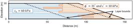
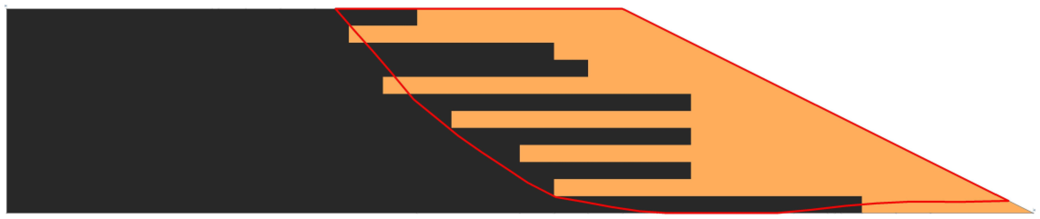
A total of 750 random component cross-sections were generated with 6, 8, 12 or 20 layers, and vertical steps positioned randomly between the layer bounds (see Figure 1). The inner bound was 75 m from the slope and the outer bound 15 m. This produced a wide range of potential upstream wall configurations. A 2D factor of safety (F_2D) was calculated for each component cross-section using the Spencer limit equilibrium method (Spencer, 1967). Rocscience Slide2 calculated F_2D using the auto-refine search method, which iteratively adjusts slip surface geometry to converge on the critical case. Figure 2 shows a typical output. This stage of modeling resulted in a distribution of F_2D reflecting the modeled stratigraphic variability.

Figure 2
Example of a 2D component cross-sections analyzed (F_2D = 0.994), black region is the inner material (c_u = 60 kPa), the orange region is the outer material (ϕ′ = 31°, c′ = 10 kPa) and the red line is the critical slip surface found.

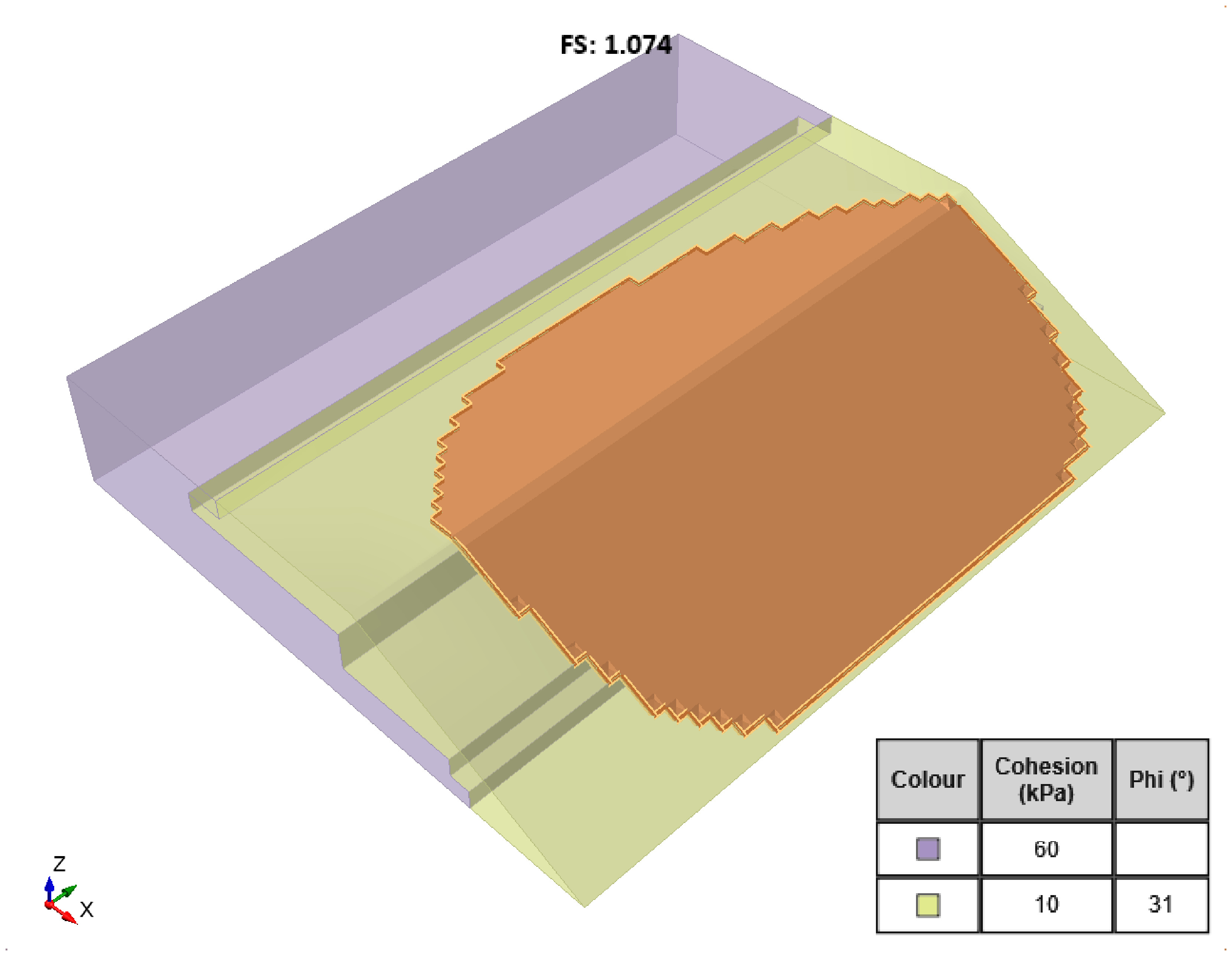
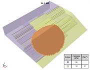
Each component cross-section was extrapolated 180 m perpendicular to the cross-section, and a 3D factor of safety (F_3D) was calculated using Rocscience Slide3 (see Figure 3). The extrapolation length was chosen iteratively to ensure that slip surfaces were not impeded by either end of the model. The Spencer limit equilibrium method, with extensions by Huang et al. (2002) and Cheng & Yip (2007), was used to determine the critical factor of safety for an ellipsoidal slip surface identified via Slide3’s cuckoo search algorithm, which employs a random walk approach. This stage of modeling produced a distribution of F_3D reflecting stratigraphic variability within each cross-section, but not along the slope’s length.

Figure 3
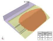
Example of a 3D component slope analyzed (F_3D = 1.074). The red zone is the identified critical slip surface.

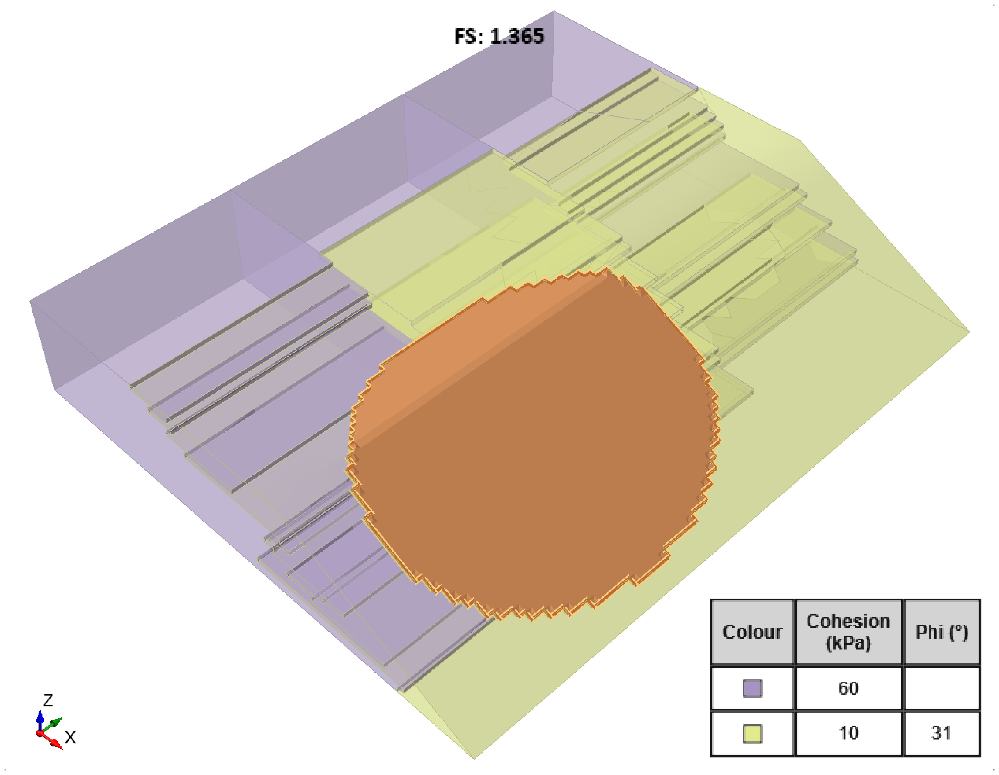
To simulate stratigraphic variability along a slope, a composite slope was created by joining three component cross-sections, each extrapolated 60 m perpendicular to the cross-section (Figure 4). The extrapolated distance was iteratively chosen so that slip surfaces were wider than a single component. Sections were systematically selected and ordered to maximize the number of unique composite slopes. End boundaries were non-periodic, meaning the search zone was confined to these three components. This produced 750 composite slopes, each of which was analyzed for a 3D factor of safety using the same Slide3 search settings. This factor of safety was assumed to represent the actual stability of the slope (F_A) with three possible F_2D and F_3D values – minimum, median and maximum – depending on the sampled section. This stage of modeling produced a distribution of F_3D reflecting stratigraphic variability within each cross-section and along the slope’s length.

Figure 4
Example of a 3D composite slope analyzed (F_A = 1.365). The red zone is the identified critical slip surface.

Composite slopes were grouped by the coefficient of variation (CV) of the three component F_2D values into three equal-sized groups: Group 1 (0% < CV ≤ 7%), Group 2 (7% < CV ≤ 11%), and Group 3 (11% < CV ≤ 25%). Table 1 provides summary statistics for each group. This shows that in addition to increasing variability within the groups the average F_2D also increased marginally (differences disappear when rounded to two significant figures). This grouping was used primarily to separate the composite slopes to help visualize how increasing variability impacted the differences between F_2D, F_3D and F_A.

Table 1
Average (M), standard deviation (SD) and coefficient of variation (CV) for all F_2D making up each group.

Group	Sample size	Summary statistics of all component F2D in sample.
		M	SD	CV
1 (0% < CV ≤ 7%)	249	1.090	0.094	9%
2 (7% < CV ≤ 11%)	249	1.100	0.110	10%
3 (11% < CV ≤ 25%)	252	1.125	0.160	14%

3. Results

3.1 Comparison of F_A to F_2D

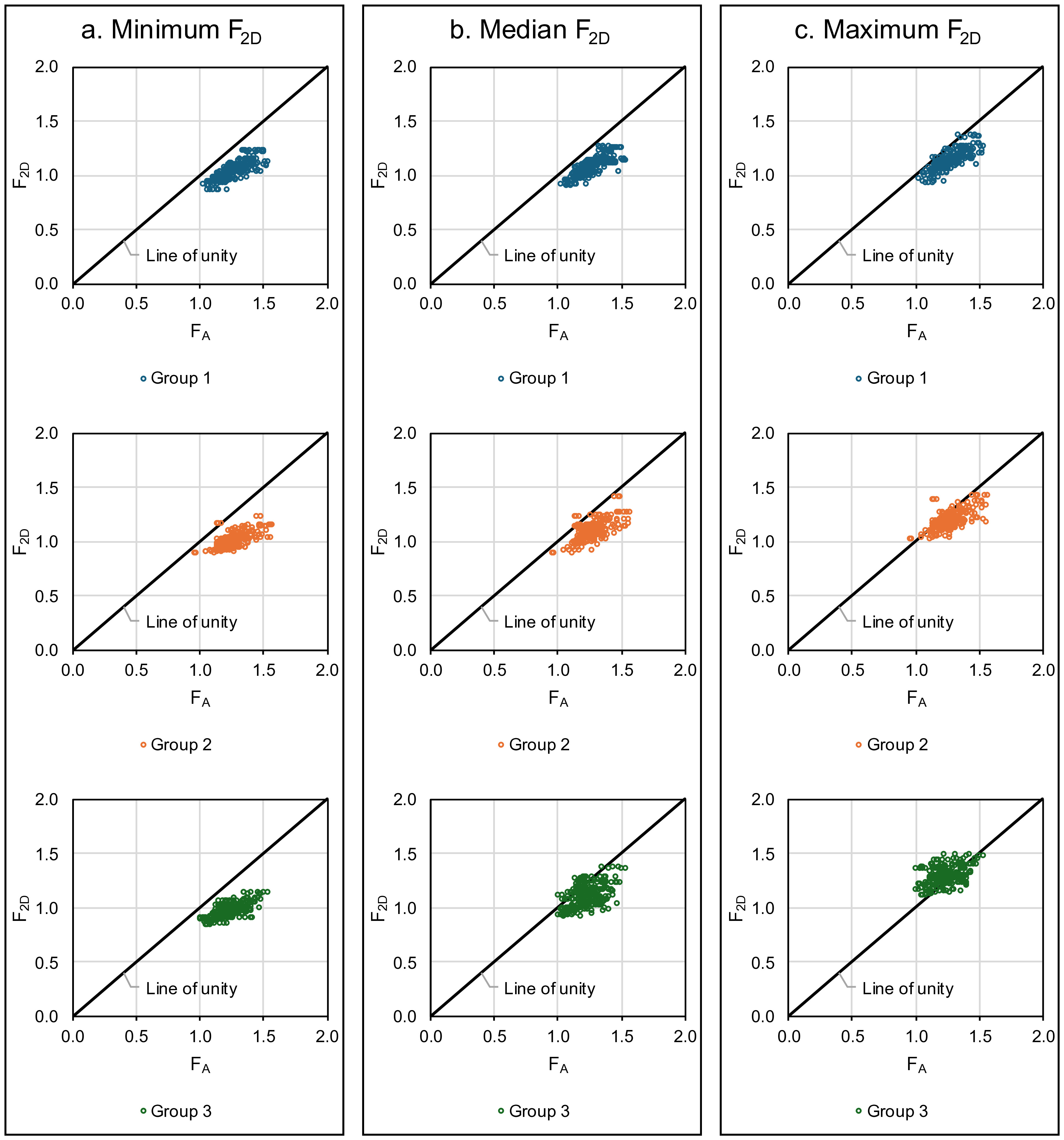
Figure 5 compares F_A (3D factors of safety incorporating stratigraphic variability along the slope’s length) to each of the three possible F_2D (2D factors of safety for component cross-sections) for the three groups of variability. Figure 5a shows that if the weakest cross-section was sampled (i.e., the cross-section that results in the minimum F_2D), the resulting 2D factor of safety was generally lower than F_A for all groups. Table 2 shows that for this weakest section, it was only for Group 2 that 1% of F_2D values were higher than F_A and therefore unsafe. The difference between F_A and Minimum F_2D increased from 0.2 to 0.3 with increasing variability. When the median section was sampled (Figure 5b), more F_2D were unconservative, particularly for higher variability, as illustrated by more Group 3 points plotting above the line of unity. For the median section, the calculated F_2D and F_A were nevertheless close, differing by between 0.1 and 0.2 (Table 2). Sampling the strongest cross-section (maximum F_2D) significantly increased the number of unsafe analyses, especially at higher variability, as shown by the large portion of Group 3 points above the line of unity in Figure 5c. Table 2 shows more than half of Group 3 had maximum F_2D exceeding F_A. Despite this, maximum F_2D values were close to F_A, with the difference ranging between -0.1 and 0.1. If we consider all F_2D, across all variability groups, 11% of F_2D were higher than F_A with the average difference between F_A and F_2D being 0.2 and the least conservative difference being -0.3.

Figure 5
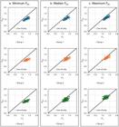
Scatter plots comparing 3D factor of safety for each composite slope to the three possible component 2D factors of safety.

Table 2
Summary statistics for 2D comparisons (Min., Median and Max. refer to the sampled cross-section).

Group	Percentage unsafe F2D			Average Δ = FA – F2D
	Min.	Median	Max.	Min.	Median	Max.
1 (0% < CV ≤ 7%)	0%	0%	0%	0.2	0.2	0.1
2 (7% < CV ≤ 11%)	1%	1%	12%	0.3	0.2	0.1
3 (11% < CV ≤ 25%)	0%	13%	69%	0.3	0.1	-0.1

3.2 Comparison of F_A to F_3D

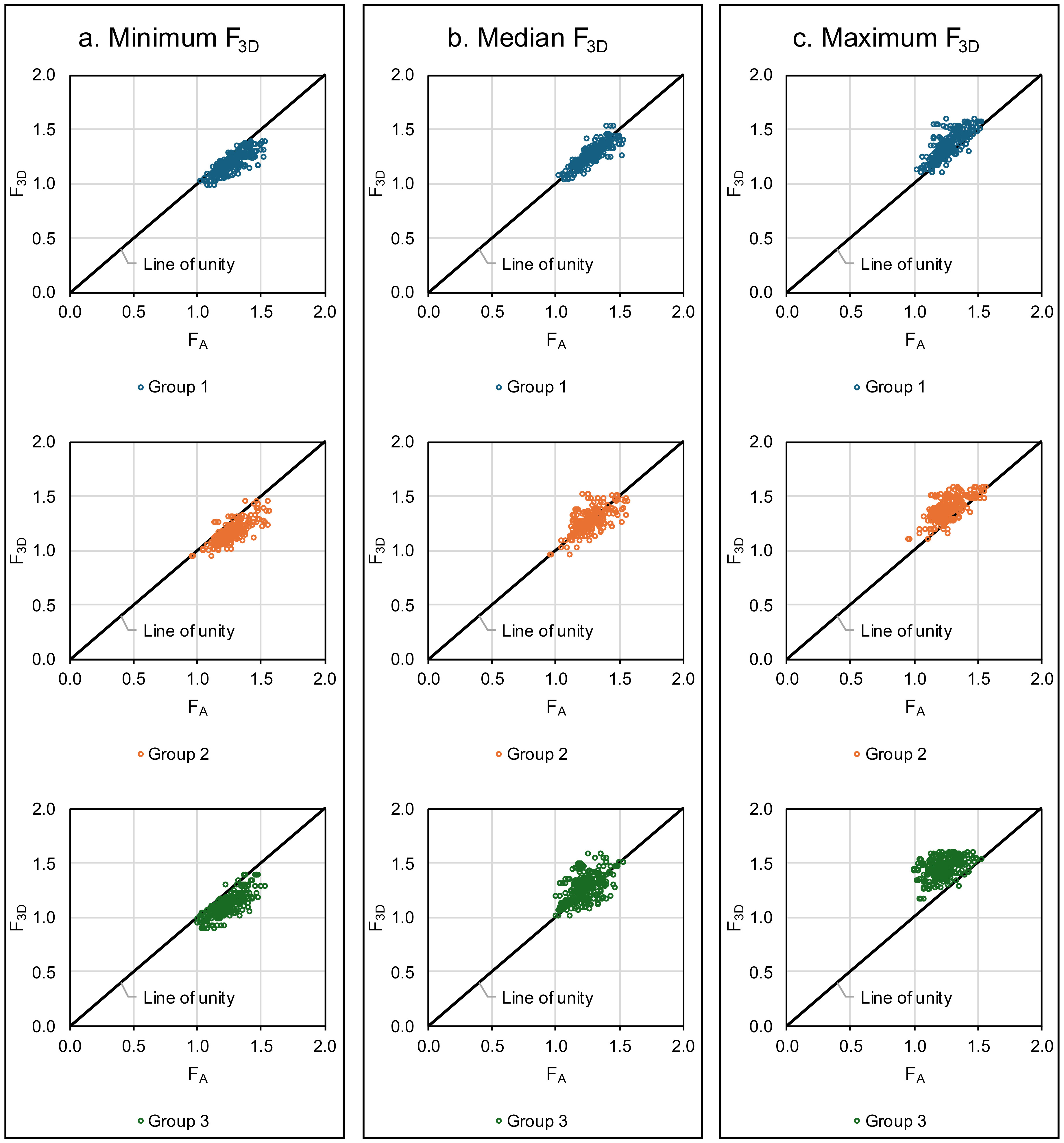
Figure 6 compares F_A (3D factors of safety incorporating stratigraphic variability along the slope’s length) to each of the three possible F_3D (3D factors of safety for component cross-sections ignoring stratigraphic variability along the slope’s length) for the three groups of variability. Figure 6a shows that sampling the weakest extrapolated cross-section (i.e., minimum F_3D) mostly resulted in a factor of safety lower than F_A for all groups. Table 3 shows that for this weakest section, between 0% and 4% of F_3D values were unsafe, with the average difference between F_A and F_3D being 0.1 for all groups. The percentage of unsafe analyses decreases with increasing variability when the weakest cross-section is sampled, whereas it increases with variability when the median and strongest cross-sections are sampled. However, this apparent contradiction arises because increasing variability also increases the strength of the median and maximum cross-sections, leading to a higher F_A. If the median section was sampled and extrapolated (Figure 6b), many resulting F_3D were unconservative, increasing from 33% to 59% with variability, as shown by more points plotting above the line of unity for Group 3 compared to Group 1. For this median section calculated F_3D and F_A were on average similar. Sampling the strongest extrapolated cross-section (i.e., maximum F_3D), resulted in most calculated F_3D being unsafe (Figure 6c). Table 3 shows that between 84% and 98% of maximum F_3D exceeded F_A, with maximum F_3D being on average between -0.1 and -0.3 away from F_A. Across all F_3D for all three variability groups, 46% of F_3D were unsafe, with the average difference between F_A and F_3D being 0.0 and the least conservative being -0.5.

Figure 6
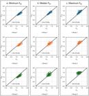
Scatter plots comparing 3D factor of safety for each composite slope to the three possible component 3D factors of safety.

Table 3
Summary statistics for 3D comparisons (Min., Median and Max. refer to the sampled cross-section).

Group	Percentage unsafe F3D			Average Δ = FA – F3D
	Min.	Median	Max.	Min.	Median	Max.
1 (0% < CV ≤ 7%)	4%	33%	84%	0.1	0.0	-0.1
2 (7% < CV ≤ 11%)	3%	45%	89%	0.1	0.0	-0.1
3 (11% < CV ≤ 25%)	1%	59%	98%	0.1	0.0	-0.2

4. Practical implications

From a practical perspective, this analysis highlights the relative safety and efficiency of carrying out 2D slope stability analysis over an extrapolated 3D slope stability analysis. Given the inherent limitations in the number of cross-sections that can be feasibly sampled on such large and variable structures, the findings offer insights into the reliability of these methods. This analysis suggests that if a single random 2D analysis is performed, there is an 11% chance that the resulting F_2D will be unsafe (i.e., the 3D factor of safety determined with stratigraphic variability would be lower). The difference in resulting F_2D relative to F_A is in the order of 0.2 (i.e., average F_A – F_2D), but in the worst-case scenario this difference is -0.3. This suggests that while 2D analyses may be generally conservative, they are not immune to significant underestimation of risk in certain conditions.

When a single 2D section is extrapolated to represent the entire 3D slope, the probability of an unsafe analysis increases to 46%. Although the average extrapolated section had an F_3D aligned with F_A, the worst-case difference is as much as -0.5. This highlights the potential danger of over-reliance on extrapolated 2D data in complex, heterogeneous environments, where localized weaknesses and stratigraphic variability may not be adequately captured by an extrapolated cross-sectional analysis.

The reason why an extrapolated 3D slope stability analysis is unconservative in many instances is that it fails to account for weak sides, toe, and back scarp conditions that exist when stratigraphic variability along the length of a slope was taken into consideration. These features can be overlooked when the analysis assumes homogeneity or relies on limited cross-sectional data. This highlights the importance of investigating conditions along the length of a slope, particularly if a 3D analysis is to be performed.

A simple assessment of the number of sections required to limit the number of unsafe analyses can be obtained by assuming sampling of cross-sections is mutually exclusive. With this simplifying assumption the decreasing probability of an unsafe analysis given additional cross-sections (P_n) is sampled can be determined using:

$P_n={(1-\left(1-P_1\right))}^n$ (1)

where P₁ = probability of unsafe analysis for one cross-section; and n = number of cross-sections.

Applying this to the data for 2D cross-section shows that to reduce 11% to 1% at least two cross-sections must be randomly sampled. In contrast, for extrapolated 3D cross-sections, reducing 46% to 1% requires at least six cross-sections to be randomly sampled. This simple probabilistic model illustrates the significantly greater data requirements for reliable 3D analyses. These probabilities should not be confused with target levels of reliability, as they are simply a means to compare, in relative terms, the amount of data required to prepare a 3D slope stability model relative to a 2D slope stability model. The limited scope of this paper does not address target reliabilities for 2D or 3D slope stability analyses.

Another key implication of this parametric study is the importance of locating the weakest cross-section for long, varying embankments like tailings dams. Each dam is unique, and practitioners need to apply suitable tools to locate this critical cross-section. Experience performing slope stability analysis suggests that some indicators of weak sections include poor drainage conditions, short seepage paths, weak foundation materials, deviations from original design geometry, inadequate beach control, residual shear zones, and sections with greater height or complex geometry. Monitoring data such as anomalous piezometric readings and displacements, as well as environmental factors like vegetation growth and animal activity, also provide valuable clues to potential instability. Tailings dams are dynamic systems, and weak zones may evolve over time due to changes in deposition, drainage, and loading.

The study also highlights the inefficiency of simply extrapolating 2D sections to estimate 3D factors of safety. Instead, resources should be allocated to investigating conditions adjacent to sections with low factors of safety. The spacing of these additional cross-sections should be based on the expected size of critical slip surfaces. This targeted approach allows for the incorporation of actual stratigraphic variability into a 3D model, thereby improving the reliability of the analysis.

5. Conclusions

This study introduces the concept of stratigraphic variability and investigates its impact on the reliability of two-dimensional (2D) and three-dimensional (3D) slope stability analysis of tailings dams. While random field theory has historically offered valuable insights into the influence of soil variability, forensic investigations and practical experience suggest that slope failures are more often governed by stratigraphic boundaries and phreatic conditions rather than by random variability alone. This underscores the need to shift analytical emphasis towards understanding and modeling stratigraphic transitions, especially in layered systems such as upstream tailings dams. The key findings and practical recommendations from this study are summarized below:

• The parametric investigation conducted in this study revealed that 2D analyses, although generally conservative, are not immune to underestimating risk. A single randomly selected 2D cross-section was found to carry an 11% probability of producing an unsafe factor of safety (i.e., the 2D factor of safety is higher than the 3D factor of safety calculated with stratigraphic variability);

• When extrapolating a 2D cross-section for 3D slope stability analysis, this study found there is a 46% likelihood of generating an unsafe factor of safety. This is because the 3D factor of safety calculated without accounting for stratigraphic variability tends to be higher than the value determined with stratigraphic variability included. This highlights the importance of investigating conditions along the crest of a tailings dam if a 3D slope stability analysis is to be performed;

• The probability of an unsafe result is greatly reduced if the factor of safety is calculated for the weakest cross-section. While several indicators for identifying weak conditions are included in the text, these are not exhaustive, and practitioners must apply their minds in their context to ensure localized weaknesses and stratigraphic variability are adequately captured.

List of symbols and abbreviations

2D Two-dimensional

3D Three-dimensional

c’ Effective cohesion

c_u Undrained shear strength

n Number of cross-sections

CV Coefficient of variation

F Factor of safety

F_2D Two-dimensional factor of safety

F_3D Three-dimensional factor of safety associated with extrapolated 2D section

F_A Three-dimensional factor of safety for a slope of three composite sections

H Unit horizontal length

L/H Slope’s length-to-height ratio

M Average

P₁ Probability of unsafe analysis for one cross-section

P_n Probability of an unsafe analysis given additional cross-sections

SD Standard deviation

V Unit vertical length

γ Specific weight

σ′ Effective stress

σ_v′ Vertical effective stress

τ Shear strength

ϕ′ Effective internal friction angle

Acknowledgements

This manuscript benefitted from fruitful discussions along the way with Prof Nico de Koker (Stellenbosch University), Dr Andrew Way (University of Pretoria) and Prof Peter Day (Stellenbosch University).

Data availability

The datasets generated and analyzed in the course of the current study are available from the corresponding author upon request.

• Discussion open until February 28, 2027.
• Declaration of use of generative artificial intelligence
  This work was prepared with the assistance of generative artificial intelligence (GenAI) Microsoft Copilot with the aim of searching for literature and editing the manuscript. The entire process of using this tool was supervised, reviewed and when necessary edited by the authors. The authors assume full responsibility for the content of the publication that involved the aid of GenAI.

References

• Albataineh, N. (2006). Slope stability analysis using 2D and 3D methods [Unpublished master’s dissertation]. University of Akron.
• Blight, G.E. (2010). Geotechnical engineering for mine waste storage facilities. London: Taylor & Francis Group.
• Chakraborty, A., & Goswami, D. (2016). State of the art: three dimensional (3D) slope-stability analysis. International Journal of Geotechnical Engineering, 10(5), 493-498.
• Chaudhary, K.B., Domingos, V.H., Gitirana Junior, G., Fredlund, M., & Lu, H. (2016). Three-dimensional slope stability: geometry effects. In Proceedings of the Tailings and Mine Waste 2016, Keystone, CO, USA. Vancouver: University of British Columbia.
• Cheng, Y., & Yip, C. (2007). Three-dimensional asymmetrical slope stability analysis extension of Bishop’s, Janbu’s, and Morgenstern-Price’s techniques. Journal of Geotechnical and Geoenvironmental Engineering, 133(12), 1544-1555.
• Donaldson, G.W. (1960). The stability of slimes dams in the gold mining industry. Journal of the Southern African Institute of Mining and Metallurgy, 61(3), 183-199.
• Duncan, J.M., Wright, S.G., & Brandon, T.L. (2014). Soil strength and slope stability. Hoboken: John Wiley & Sons.
• Fell, R., Macgregor, P., Stapledon, D., Bell, G., & Foster, M. (2015). Geotechnical engineering of dams (2nd ed.). London: CRC Press.
• Griffiths, D., & Marquez, R. (2007). Three-dimensional slope stability analysis by elasto-plastic finite elements. Geotechnique, 57(6), 537-546.
• Hicks, M., Chen, J., & Spencer, W. (2008). Influence of spatial variability on 3D slope failures. In Proceedings of the 6th International Conference on Computer Simulation in Risk Analysis and Hazard Mitigation (pp. 335-342), Thessaly, Greece. Southampton: WIT Press.
• Hicks, M.A., & Li, Y. (2018). Influence of length effect on embankment slope reliability in 3D. International Journal for Numerical and Analytical Methods in Geomechanics, 42(7), 891-915.
• Hicks, M.A., & Spencer, W.A. (2010). Influence of heterogeneity on the reliability and failure of a long 3D slope. Computers and Geotechnics, 37(7-8), 948-955.
• Huang, C.C., Tsai, C.C., & Chen, Y.H. (2002). Generalized method for three-dimensional slope stability analysis. Journal of Geotechnical and Geoenvironmental Engineering, 128(10), 836-848.
• Li, Y., Hicks, M.A., & Nuttall, J.D. (2013). Probabilistic analysis of a benchmark problem for slope stability in 3D. In Proceedings of the 3rd International Symposium on Computational Geomechanics (pp. 641-648), Krakow, Poland.
• Lim, K., Li, A., & Lyamin, A. (2015a). Three-dimensional slope stability assessment of two-layered undrained clay. Computers and Geotechnics, 70, 1-17.
• Lim, K., Li, A., Lyamin, A., & Cassidy, M. (2015b). Slope stability analysis for fill slopes using finite element limit analysis. In Proceedings of the XVI ECSMGE Geotechnical Engineering for Infrastructure and Development, Edinburgh. London: ICE Publishing.
• Liu, Y., Zhang, W., Zhang, L., Zhu, Z., Hu, J., & Wei, H. (2018). Probabilistic stability analyses of undrained slopes by 3D random fields and finite element methods. Geoscience Frontiers, 9(6), 1657-1664.
• MacRobert, C.J., & Blight, G.E. (2013). A field study of the in situ moisture regime during active hydraulic tailings deposition. Journal of the South African Institution of Civil Engineers, 55(3), 57-68.
• Michalowski, R.L. (2010). Limit analysis and stability charts for 3D slope failures. Journal of Geotechnical and Geoenvironmental Engineering, 136(4), 583-593.
• Olson, S.M., & Stark, T.D. (2003). Yield strength ratio and liquefaction analysis of slopes and embankments. Journal of Geotechnical and Geoenvironmental Engineering, 129(8), 727-737.
• Seed, R.B., Mitchell, J.K., & Seed, H.B. (1990). Kettleman hills waste landfill slope failure. II: stability analyses. Journal of Geotechnical Engineering, 116(4), 669-690.
• Spencer, E. (1967). A method of analysis of the stability of embankments assuming parallel inter-slice forces. Geotechnique, 17(1), 11-26.
• Varkey, D., Hicks, M.A., & Vardon, P.J. (2017). Influence of spatial variability of shear strength parameters on 3D slope reliability and comparison of analysis methods. In Proceedings of the Geo-Risk 2017 (pp. 400-409), Denver, CO. ASCE.
• Varkey, D., Hicks, M., & Vardon, P. (2018). 3D slope stability analysis with spatially variable and cross-correlated shear strength parameters. In Proceedings of the 9th European Conference on Numerical Methods in Geotechnical Engineering (NUMGE 2018) (Vol. 1), Porto, Portugal. CRC Press.
• Vick, S.G. (1990). Planning, design, and analysis of tailings dams. Vancouver: BiTech Publishers Ltd.
• Wu, C., Wang, Z.Z., Goh, S.H., & Zhang, W. (2024). Comparing 2D and 3D slope stability in spatially variable soils using random finite-element method. Computers and Geotechnics, 170, 106324.
• Zhang, L., Gong, W.-P., Li, X.X., Tan, X.H., Zhao, C., & Wang, L. (2022). A comparison study between 2D and 3D slope stability analyses considering spatial soil variability. Journal of Zhejiang University. Science A, 23(3), 208-224.

Edited by

• Editor:
  Renato P. Cunha https://orcid.org/0000-0002-2264-9711

Publication Dates

• Publication in this collection
  31 July 2026
• Date of issue
  2026

History

• Received
  11 Aug 2025
• Accepted
  22 Apr 2026