Identification of a time-varying SIR Model for COVID-19

ABSTRACT

Throughout human history, epidemics have been a constant presence. Understanding their dynamics is essential to predict scenarios and make substantiated decisions. Mathematical models are powerful tools to describe an epidemic behavior. Among the most used, the compartmental ones stand out, dividing the population into classes with well-defined characteristics. One of the most known is the SIR model, based on a set of differential equations describing the rates of change of three categories over time. These equations consider parameters such as the disease transmission rate and the recovery rate, which both change over time. However, typically models use constant parameters and can not describe the behavior of a disease over long periods. In this work, it is proposed a method to estimate the parameters of a SIR model with a time-varying transmission rate, based on an optimization problem that minimizes the sum of the squares of the errors between the model and historical data. Additionally, based on the infection rates determined by the algorithm, the model’s ability to predict disease activity in future scenarios was also investigated. Epidemic data released by the government of the State of Rio Grande do Sul in Brazil was used to evaluate the models. The models showed a very good forecasting ability, resulting in errors for predicting the total number of accumulated infected persons of 0.13% for 7 days ahead and 0.6% for 14 days ahead.

Keywords:
COVID-19; simulation; identification; prediction

1 INTRODUCTION

Humanity has coexisted with infectious diseases since the beginning of the history. Some of these infirmities can simultaneously reach a large number of individuals in the same area. When these outbreaks of contamination occur, that place is facing an epidemic. The prevalence and effects of an epidemic can diversify a lot. In less developed countries, even low-risk diseases may have serious consequences. Economic development defines, in general, the quality of health care and the efficiency of watching and containing an infectious disease. Because of that, worrying rates of mortality are still registered for malaria, typhus, cholera, and other easily treatable infirmities⁵. Furthermore, an epidemic situation can affect the economy of some regions. In some cases, control measures change people’s circulation and the operation of commercial establishments, generating a negative economic impact during the application of these measures. Therefore, understanding the phenomenon is crucial to determine actions to fight against this problem.

Mathematical modeling is an extremely useful tool to describe different events³. It can simulate the activity of a system that reproduces, for example, the dynamics of an infectious disease. Then, it’s possible to analyze and interpret the results, looking for ways to control epidemics¹⁶. An accurate model enables political and sanitary authorities to adopt based decisions.

In literature, several epidemic models are currently used. Among them, compartmental ones stand out, dividing the population into classes with common characteristics and establishing their relations¹⁸. One of them is the SIR model, which divides the population into three classes and proposes a set of differential equations that define the rate of change of each compartment over time⁴. This change is directly linked to the parameters that make up the equations, as they represent rates that describe the dynamics of disease spread in the population. Typically, the differential equations of the SIR model use these constants to describe how the number of individuals in each compartment (susceptible, infected, and removed) varies over time. However, for long periods, assigning a single value to these parameters may not be effective. Changes in population behavior, government measures, and even the nature of the disease can alter during this period. Thus, the model’s ability to reproduce the disease dynamics is compromised.

In¹⁹, a discussion is presented on the difficulty of obtaining effective COVID-19 predictions using epidemiological models. The authors analyzed the reasons behind the wide variability in results, concluding that this is due to the failure to identify the necessary parameter calibrations for the system. They then evaluated the use of two compartmental models, SIR and SEIR, to represent the information contained in confirmed case data. They demonstrated that the SIR model performs better and that simpler models can be more reliable than more complex ones. To illustrate this, they modeled the impacts of quarantine in Wuhan, China, and a potential second outbreak after its conclusion.

The article¹⁷ presents a review of various publications involving mathematical modeling and the use of artificial intelligence to understand COVID-19 dynamics. A total of 61 journal articles were studied, revealing the widespread use of compartmental models, particularly SIR and SEIR. Regarding AI implementations, neural networks stood out. The authors concluded that both mathematical modeling and artificial intelligence have proven to be reliable tools for understanding the pandemic.

In the 2022 study¹⁰, the reasons behind the failure of some COVID-19 predictions were investigated. The authors concluded that incorrect modeling, lack of transparency, erroneous data, and the absence of evidence on the effects of interventions are among the main causes. They emphasize that careful modeling, which respects the disease’s unique characteristics, and model validation are crucial to avoiding errors. Additionally, they advocate for major decisions to be based on global evidence rather than specific cases.

In¹¹, a discrete SIR model was used to estimate the prevalence of the COVID-19 virus, combining different available data sources, such as deaths, confirmed cases, and positive tests. Using a Bayesian framework, the model was calibrated to project the number of new infections in the states of Ohio and Indiana, in the United States. As a result, the authors found that the number of infections was underestimated, particularly at the beginning of the pandemic.

Models with time-varying parameters have been proposed to describe infectious diseases, to deal with this problem^{13), (15}. The article¹⁴ proposes a time-varying model that assumes a decaying infecting rate, which is only valid for short periods. The article²⁰ proposes an MCMC algorithm that is highly computationally intensive, and is capable of computing a value for each week, but incapable of computing daily estimates. On the other hand, article⁷ presents a method to estimate the infection rate directly from data, that is only capable of obtaining daily estimates. In this article, we propose a new method for identifying a time-varying SIR model that is computationally efficient and capable of estimating the infection rate of the disease for any time interval, whether they are daily, weekly or monthly.

We have used data from the first 770 days of the COVID-19 pandemic in the state of Rio Grande do Sul in Brazil to evaluate the proposed algorithm. An optimization algorithm was then applied to minimize the squared difference between the total infected reported by the data and that simulated by the model. However, it was found that the large number of elements in the vector posed difficulties in this identification. Therefore, a strategy was devised to gradually increase the number of entries in the vector, allowing the algorithm to converge to the desired solution. Based on the obtained results, the real behavior of the pandemic in the state of Rio Grande do Sul was compared with that simulated by the identified model.

After identifying the model and its ability to describe the pandemic’s behavior over a long period, its validity in predicting disease activity in future periods was also assessed. For this purpose, the effectiveness of the model in predicting disease behavior in scenarios 7, 14, 30, 60, and 180 days ahead was evaluated. To achieve this, the percentage error between the accumulated number of infected individuals in the period and the simulated value from the model identification was calculated.

This article is disposed as follows: In the next section, a simplified SIR compartmental model is presented, defining its configuration in a differential equations system and explaining its dynamics. The simulation of this model is also displayed. Then, in Section 3, the identification of this model based on data provided by the state government will be shown. After, in Section 4, the validity of the model to predict the pandemic behavior in future scenarios will be verified. Finally, in Section 5, discussions about the results are made, with the appropriate conclusions.

2 SIR MODEL

Mathematical models are important tools to describe and control infectious diseases. In literature, the most used are the compartmental ones, that separate populations into classes¹⁶. These compartments represent the individuals involved in the process and the state in which they find themselves.

The choice of the model should take into account disease properties, such as how it spreads in the population¹⁶. A model with lots of compartments could potentially describe better a disease, but usually results in poor predictions due to the complexity of the model and difficulty in correctly estimating the large number of parameters⁸. Usually, reduced order models with two to four compartments, and few parameters, result in better predictions and are preferred to describe infectious diseases.

The SIR model was developed by Kermack and McKendrick¹³ and proposes a simple but efficient configuration to represent diseases with community transmission, those whose origin of infection is undetermined because the transmitting agent circulates throughout the population. The model suggests to express the system behavior by three groups:

• Susceptible (S): Population that can be infected if they have any contact with the disease;

• Infected (I): Individuals who are sick and are capable of infecting susceptible;

• Removed (R): People who are no longer infected and can’t infect any individual anymore. This group is composed of recovered or dead.

In that perspective, total population N is considered constant and given by the sum S(t)+I(t)+R(t)=N. The dynamics imply that susceptible people are subject to infection when they have contact with an individual from the infected class. Then, they become part of the infected group for a while, when finally don’t carry the disease anymore (cure or death) and become part of the removed group. This process can be schematized as follows:

$S\to I\to R$

A configuration for a SIR model is expressed by a set of ordinary differential equations:

$\left\{\begin{array}{c}\frac{dS\left(t\right)}{dt}=-\frac{\beta I\left(t\right)S\left(t\right)}{N}\\ \frac{dI\left(t\right)}{dt}=\frac{\beta I\left(t\right)S\left(t\right)}{N}-\gamma I\left(t\right)\\ \frac{dR\left(t\right)}{dt}=\gamma I\left(t\right)\end{array}\right.$ (2.1)

Notice that in the first equation, which denotes the variation rate of susceptible, contamination of individuals is given by the interaction between S and I classes. It is assumed that each individual in the susceptible group has, on average, e encounters with other people every day and that the probability of a person being in the infected group is $\frac{I\left(t\right)}{N}$. It is also assumed that each encounter between a person from the susceptible group and another person from the infected group has a probability p of infecting the susceptible person. The parameter β=e·p encompasses both the average number of encounters e and the probability p and varies with the development of the epidemic, because people change their behavior towards the disease and the disease changes over time. At the same rate that the susceptible population leaves the S class, it enters the I class. Similarly, a portion of the infected population leaves this class, after a mean period $\frac{1}{\gamma }$, and becomes part of the removed group R.

2.1 Analytical Solution

One of the goals of using mathematical models for epidemic situations is to determine how the disease is spreading. For this purpose, it is interesting to observe the system’s behavior over time, motivating oneself to check when the spread will begin to decline.

The SIR model does not have an analytical solution, but one can attempt to understand the evolution of an epidemic through this model when the disease propagation is in its early stages. If, at the beginning of the process (t=0), the number of susceptible individuals is almost the entire population (S≈N), and taking I(0)=I ₀>0, then in the second equation:

$\frac{dI\left(t\right)}{dt}=\beta I\left(t\right)-\gamma I\left(t\right)=I\left(t\right)\left(\beta -\gamma \right),$ (2.2)

whose solution can be easily found using the method of separation of variables, resulting in:

$I\left(t\right)=I_0{e}^{\left(\beta -\gamma \right)t}=I_0{e}^{\gamma t\left(\frac{\beta }{\gamma }-1\right)}$ (2.3)

Given that $R_0=\frac{\beta }{\gamma }$, it follows that:

• Se R ₀>1, I(t)→∞, that is, epidemic continues to grow;

• Se R ₀<1, I(t)→0, that is, the infection tends to end over time.

The constant R ₀ is called the infection reproduction rate.

2.2 Time-varying infection rate SIR model

The infection rate of the conventional SIR model represents both: the probability of a susceptible person contracting the disease when coming into contact with an infected individual and the mean number of encounters a susceptible person has with other people every day. This rate is crucial for understanding how a disease spreads over time. However, assigning a fixed value to this parameter for an extended period can lead to inaccuracies when attempting to simulate the behavior of a disease. This can occur because the model depends on the interaction between susceptible and infected classes. Such interaction may change if a long period is considered. Individuals may alter their behavior as the disease spreads, changing the chance of infection. There’s also the possibility that authorities may take containment measures, preventing greater contact between individuals in these two classes. Not to mention, the disease itself may mutate, becoming more or less contagious, thereby increasing or decreasing the likelihood of someone contracting it.

From this, an alternative SIR model can be used, with a time-varying infection rate¹⁵. This allows defining how the disease is spreading on a daily, weekly, or monthly basis. To achieve this, the parameter β is modified so that instead of receiving a fixed value, it is function over time. Thus, the model is configured as follows:

$\left\{\begin{array}{c}\frac{dS\left(t\right)}{dt}=-\frac{\beta \left(t\right)I\left(t\right)S\left(t\right)}{N}\\ \frac{dI\left(t\right)}{dt}=\frac{\beta \left(t\right)I\left(t\right)S\left(t\right)}{N}-\gamma I\left(t\right)\\ \frac{dR\left(t\right)}{dt}=\gamma I\left(t\right),\end{array}\right.$ (2.4)

where β(t) is the time-varying infection rate at time t.

The cumulative number of infected individuals is defined by:

$\hat{Y}\left(t,\beta \left(t\right)\right)={\int }_0^t\frac{\beta \left(\tau \right)I\left(\tau \right)S\left(\tau \right)}{N}d\tau =N-S\left(\tau \right)$ (2.5)

where we have explicitly defined $\hat{Y}$ as a function of time t and the time-varying infection rate β(t).

2.3 Simulation of the Model

Since the model does not have an analytical solution, a computational method can be used to obtain the numerical solution of the system of differential equations that characterizes the model SIR. The one chosen in this work was the fourth-order Runge-Kutta¹², which solves a problem of the type y’(t)=f(t, x). The sampling period used was fixed, simulating the system’s behavior daily to align with the way the data is usually collected. Additionally, since the average infection period is given by 1/γ, as seen earlier, this constant can be fixed, knowing that, on average, this period is 10 days². Thus, it was assumed that γ=0.1, and, consequently, the simulated SIR model is given by:

$\left\{\begin{array}{c}\frac{dS\left(t\right)}{dt}=-\frac{\beta \left(t\right)I\left(t\right)S\left(t\right)}{N}\\ \frac{dI\left(t\right)}{dt}=\frac{\beta \left(t\right)I\left(t\right)S\left(t\right)}{N}-0.1I\left(t\right)\\ \frac{dR\left(t\right)}{dt}=0.1I\left(t\right).\end{array}\right.$ (2.6)

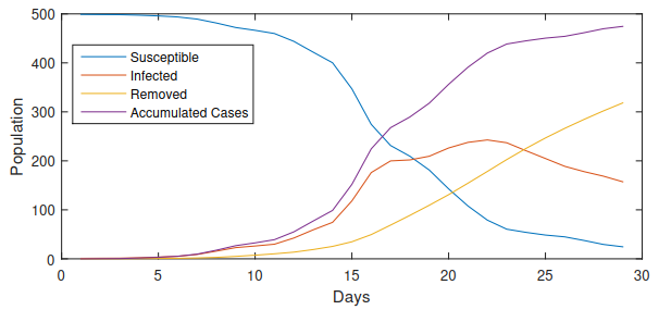
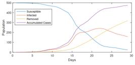
To illustrate the simulated model, the algorithm was executed in a hypothetical case for a population of N=500 over 1 month, with randomly varying daily rates, which were drawn from a uniform distribution between 0 and 1. The result can be observed in Figure 1.

Figure 1
Simulation of the time-varying SIR model.

3 IDENTIFICATION OF TIME-VARYING PARAMETER β(T)

The main result of this work is a mathematical method for the identification of the time-varying parameter β(t). Parameter identification involves, based on collected data about the studied phenomenon, estimating the values of parameters, in order to approximate the model’s behavior to the studied system⁶. To achieve this, an optimization algorithm is proposed here.

The proposed method aims to estimate the parameters that minimize the sums of a squared function²¹. This function represents the error between the solution computed by the model and the data that represents the reality. Thus, let Y(t) be the total accumulated infected at the day t and $\hat{Y}\left(t\right)$ be the simulated output of the model at the day t, the function to be optimized is defined as:

$J\left(\beta \left(t\right)\right)=\sum _{t=1}^M{\left(Y\left(t\right)-\hat{Y}\left(t,\beta \left(t\right)\right)\right)}^2$ (3.1)

where M is the number of days of the collected data. In order to compute $\hat{Y}\left(t,\beta \left(t\right)\right)$ a 4th order Runge-Kutta method is used with the following initial conditions:

$\left[\begin{array}{c}S\left(0\right)\\ I\left(0\right)\\ R\left(0\right)\end{array}\right]=\left[\begin{array}{c}N-1\\ 1\\ 0\end{array}\right],$ (3.2)

which describes the disease from the day the first person is infected on a region.

We propose the following optimization problem

$\widehat{\beta \left(t\right)}=\underset{\beta \left(t\right)}{argmin}J\left(\beta \left(t\right)\right).$ (3.3)

It is very difficult to find the solution of this optimization problem since β(t) is continuous and J(β(t)) is in general nonconvex. In this work, we propose to parametrize the function β(t) with a finite number of parameters and we also propose a clever optimization procedure to improve the convergence to the global minimum of the optimization criterion J(β(t)).

3.1 Finite Parametrization of β(t)

The function β(t) is parametrized as a piecewise constant function such that it varies periodically, but it is constant during one period:

$\beta \left(t\right)=\left\{\begin{array}{c}{\beta }_1,0\le t<t_1\\ {\beta }_2,t_1\le t<t_2\\ {\beta }_3,t_2\le t<t_3\\ ⋮\\ {\beta }_m,t_{m-1}\le t\le t_m\end{array}\right.$

and

$t_j=j·T,forj=1,2,...,m.$

and T is the period that the infection rate is kept constant. The constant T is typically set as one day, one week or one month.

In order to simplify the notation, we have grouped all the parameters as a vector

$B=\left[{\beta }_1,{\beta }_2,...,{\beta }_{m-1},{\beta }_m\right]$ (3.4)

such that the optimization problem (3.3) becomes finite:

$\hat{B}=\underset{B}{argmin}J\left(B\right)$ (3.5)

Despite the optimization problem (3.5) being finite, it is still very difficult to find the optimal solution since the objective function is nonconvex. Attempts to solve directly this problem using commercial solvers usually fail, resulting in convergence to local minima of the problem, which results in solutions that do not resemble the actual data. In the next section, we describe an iterative algorithm to solve this problem.

3.2 Optimization Algorithm

The objective of this section is to describe an iterative algorithm to solve the optimization problem (3.5).

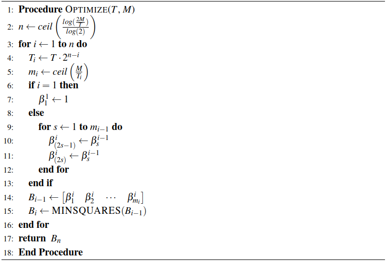
The algorithm assumes that initially, the vector B had only one element, meaning the algorithm would calculate only one value to approximate the model’s behavior to reality as if it were a single rate for the entire period. Thus, β is constant and the optimization algorithm was executed. Obviously, the error in this first iteration is large. So, the second step consists of duplicating the number of parameters and assigning to them initially the values found by the algorithm in the first optimization. In this way, the resulting error is still significant, but the result shows a better fit compared to the previous one. Thus, with each simulation, the number of elements in the vector is doubled, and it was found that the precision improves at each iteration. In fact, at some iterations, the number of parameters does not need to be exactly doubled, and some parameters may be discarded. We will describe the algorithm in detail in the sequence.

In order to compute the number of iterations, we need to find the smallest integer n such that:

$T·2^{n-1}>M.$

The solution of this inequality is:

$n=ceil\left(\frac{\log \left({\displaystyle \frac{2M}{T}}\right)}{\log \left(2\right)}\right)$

For instance, if T=7 (one week) and M=770 days then n=8 and therefore the algorithm will run 8 iterations.

On every iteration, we set i as the iteration number and define the period of this iteration as

$T_i=T·2^{n-i}.$

Then we can compute the number of sub-functions that will compose our piecewise constant function, computing the smallest integer m _i that respects:

$m_i·T_i>M.$

The solution of this inequality is:

$m_i=ceil\left(\frac{M}{T_i}\right)$

We then define β(t)=β_i (t) as piecewise constant function with m _i sub-functions:

${\beta }_i\left(t\right)=\left\{\begin{array}{c}{\beta }_1^i,0\le t<t_1\\ {\beta }_2^i,t_1\le t<t_2\\ {\beta }_3^i,t_2\le t<t_3\\ ⋮\\ {\beta }_{m_i}^i,t_{m_{i-1}}\le t<t_{m_i}\end{array}\right.$

and

$t_j=j·T_i,forj=1,2,...,m_i.$

For instance, consider that T=7 (one week) and M=770 days such that the number of iterations is n=8.

At every iteration the optimization problem (3.5) is solved with

$B=\left[{\beta }_1^i,{\beta }_2^i,...,{\beta }_{m_i}^i\right].$

At the first iteration the algorithm has to find only one parameter, and it’s initial value is chosen as 1

$B=\left[1\right].$

At every other iteration, the optimization algorithm is initialized with the solution of the previous optimization problem, such that

${\beta }_{\left(2s-1\right)}^i={\beta }_{\left(2s\right)}^i={\beta }_s^{i-1},m=1,2,...,m_{i-1}.$

Table 1
Iterative strategy to solve the optimization problem.

Iteration	Period	Number of parameters
i=1	T1=896 days	m1=1
i=2	T2=448 days	m2=2
i=3	T3=224 days	m3=4
i=4	T4=112 days	m4=7
i=5	T5=56 days	m5=14
i=6	T6=28 days	m6=28
i=7	T7=14 days	m7=55
i=8	T8=7 days	m8=110

The complete algorithm may be summarized on the pseudo-code described below. The subprocedure MINSQUARES (B _i-1 ) solves the optimization problem (3.5) with initial values given by vector B _i-1 . This procedure returns B _i which is a vector composed of the β values. We have used the MATLAB software to solve this optimization problem with the function fmincon.

Algorithm 1
Optimize

3.3 Data

To perform the identification of the model parameters, data provided by the Health Department of the State of Rio Grande do Sul were used, obtained through its website¹. These data are categorized for each infected person, providing the case registration date and additional information such as gender, age, etc. The considered period spanned 770 days (or 110 weeks), starting from the first registered case.

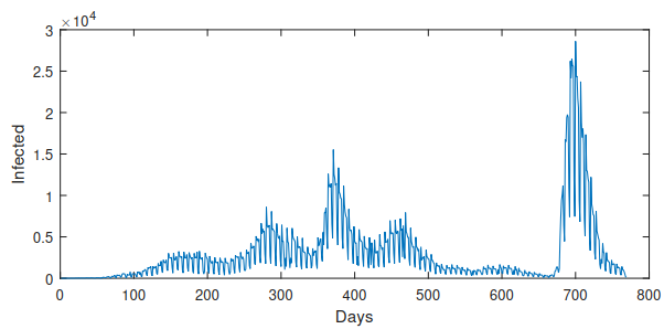
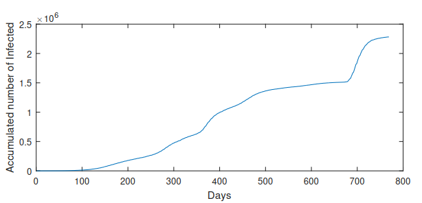
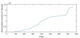
Based on these records, the software MATLAB was utilized to create graphs illustrating the number of detected cases each day, as well as the cumulative number of infected individuals over this period. This allowed the observation of the pandemic’s progression in the state, analyzing critical periods, growth, and decline in the number of cases, among other considerations. Such behaviors can be observed in the Figures 2 e 3. From there, it is possible to perform the model identification, as seen earlier, and the results are displayed in the next subsection.

Figure 2
Number of daily cases in RS state.

Figure 3
Accumulated number of cases in RS state.

3.4 Identification of a model from data

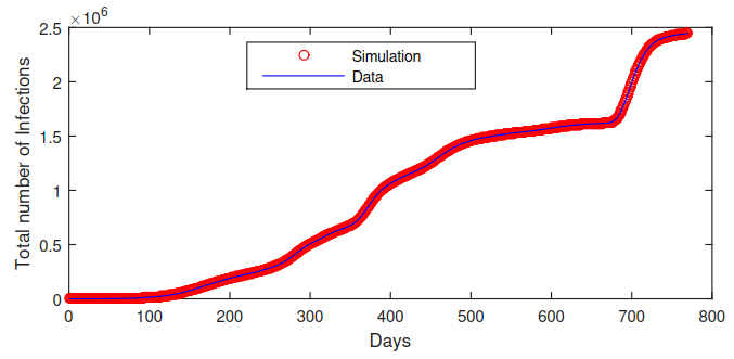
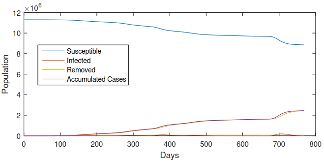
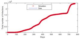
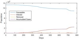
The optimization algorithm proposed in section 3.2 runs with data from section 3.3. We choose T=1 day and set M=770 days, in order to obtain a daily time-varying model. As a result, the model achieved the intended accuracy, as seen in Figure 4, where the graphs are compared. Simulating the model based on the identified rates, the system’s behavior is observed in Figure 5.

Figure 4
Real Behavior x Simulated.

Figure 5
Simulation with identified infection rates.

4 PREDICTION OF A SIR MODEL

With the use of the data, it was possible to determine the infection rates for each day of the pandemic, allowing the behavior and evolution of infections to be observed with good precision.

However, this technique reveals what happened in the past. Is it possible to understand how this behavior will unfold in the future? Motivated by this question, an investigation was carried out to assess how effectively this model is to predict the disease activity in the days following the known data.

In this work, the aim is to determine how accurate the prediction of the SIR model can be based on the identification of its infection rates. Thus, given the behavior of the cumulative infected individuals in the previous section, the accuracy of the model in forecasting its activity over different time intervals was assessed.

4.1 Results

The process for evaluating the model at future time intervals was carried out as follows: it was assumed that the pandemic was already on its 100th day and that the infection rate for each 100 day of the pandemic was estimated. In order to estimate the following days of the pandemic, it was assumed that from that day on, the value β(t) would be constant, for t>100. Since it was known that the infection rate would change in the future, it was certain the model would be accurate in the following days but it would diverge in the future. The goal is then to determine the accuracy of the model in predicting the cumulative behavior of the pandemic over the next 7, 14, 30, 60, and 180 days. The percentage of error was computed as follows

$e_T\left(t\right)=\frac{Y\left(t+T\right)-\hat{Y}\left(t+T\right)}{Y\left(t+T\right)}$

where T={7, 14, 30, 60, 180}, such that five metrics were evaluated.

Subsequently, the same procedure was repeated starting from the 101st day, analyzing the simulation for the same subsequent periods (7, 14, 30, 60, and 180 days). This process was then repeated starting from the 102nd day and continued successively. The analysis was conducted by examining the percentage error between the prediction attempt and the previously identified behavior, as given by: For each time interval, the average percentage error and standard deviation were also computed.

4.1.1 Prediction for T=7 days

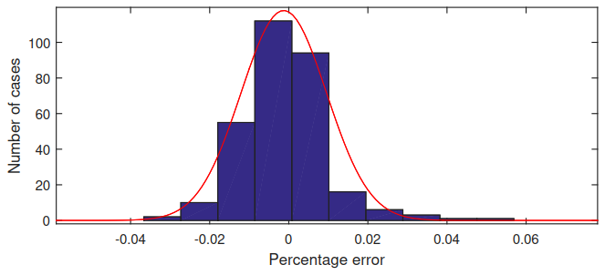
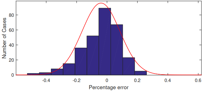
As reported earlier, the percentage error was examined between the identified model’s cumulative number of infected individuals and the data, 7 days ahead. These errors were tallied and distributed in a histogram. Additionally, the average percentage error of all simulations, along with its standard deviation, was calculated to subsequently compare the histogram with the Gaussian curve.

As can be seen, the prediction of infection rates 7 days ahead exhibited a behavior close to that of the Gaussian curve, with a calculated mean of the percentage errors at 0.13% and a standard deviation of 1.08%. As noted, the majority of cases are within one standard deviation of the mean, indicating the model’s good accuracy in forecasting the pandemic’s behavior one week into the future.

Figure 6
Percentage error 7 days in future.

4.1.2 Prediction for 14 days

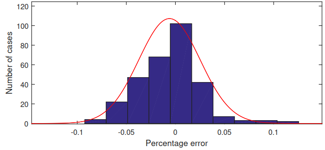
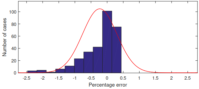
After verifying the effectiveness of the model in predicting the evolution of the pandemic one week ahead, we sought to analyze its performance two weeks into the future. The graph in Figure 7 illustrates the percentage errors of the simulations.

Figure 7
Percentage error 14 days in future.

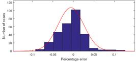
Knowing that the mean of the percentage errors was 0.6% and the standard deviation was 3.13%, it is possible to observe that, once again, the histogram’s behavior resembled a Gaussian curve. However, a higher number of simulations with errors exceeding one standard deviation from the mean were noticed, indicating that the model’s accuracy was not as good as in the previous situation.

4.1.3 Prediction for 30 days

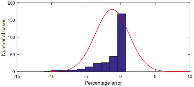
Here, the percentage error produced by the model in attempting to simulate the pandemic activity one month into the future was examined. This resulted in an average percentage error of 3.95%, with a standard deviation of 12.48%. Thus, it can be observed that, despite the average not being high, there were many cases far from the mean, and the distribution of cases did not resemble that of the Gaussian curve, as can be seen in Figure 8.

Figure 8
Percentage error 30 days in future.

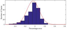
Thus, it is understood that the model did not exhibit fidelity to the actual behavior of the pandemic when attempting to predict it 30 days ahead.

4.1.4 Prediction for 60 days

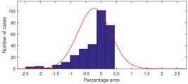
In this subsection, the results of the model simulation in attempting to predict the evolution of the cumulative number of infected individuals in the 60 days following the already known period are presented. It was determined that the average percentage error of the simulated behavior, in comparison to the actual data, was approximately 22.97%, indicating a low level of precision. Additionally, the standard deviation found was 53.32%.

When comparing the number of cases distributed in the histogram with its Gaussian curve, it is observed that there is no proximity between the graphs, as illustrated in Figure 9 Therefore, it is evident that the model is not reliable in predicting how the pandemic will unfold two months into the future.

Figure 9
Percentage error 60 days in future.

4.1.5 Prediction for 180 days

After realizing that the model did not exhibit accuracy in simulating the behavior of the pandemic for 1 or 2 months into the future, a new test was conducted to assess its activity 6 months ahead. As expected, it was observed that the percentage error was significantly high in practically all cases, as can be seen in Figure 10, depicting the distribution of cases in this scenario alongside the corresponding Gaussian curve.

Figure 10
Percentage error 180 days in future.

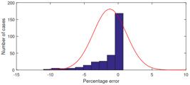
For this case, the average percentage error was 123%, with a standard deviation of 242%, confirming the impracticality of using the model to predict the disease’s behavior during this time period.

5 CONCLUSIONS

Epidemics are phenomena that frequently arise in populations. Understanding the dynamics of diseases that manifest collectively is crucial for implementing prevention and combat measures⁹. In this regard, mathematical models emerge as useful tools for this purpose.

In this study, the use of a simplified compartmental model SIR was proposed to describe the behavior of the coronavirus pandemic. However, the conventional system of differential equations in this model suggests constants with fixed values to represent the infection rate, which can lead to inaccuracies in simulating long periods. Because of this, a time-varying infection rate was adopted to reflect the daily activity of the disease. Thus, for each day, a value for this constant was identified.

In this identification, data on the population infected by SARS-CoV-2 over a period of 770 days in the state of Rio Grande do Sul were used. An optimization algorithm, based on the method of least squares, was executed to determine the infection rates on each day of analysis. Since the daily simulation required a vector with many parameters and the optimization problem was non-convex, it was necessary to develop an iterative algorithm that doubled the number of elements in the vector to be identified after each iteration.

This approach allowed for adjusting the model to the data and obtaining good accuracy in representing the accumulated number of infected individuals, as observed in the graphs comparing the simulation with the real behavior generated by the data. The identified model has very good accuracy and represents very well the development of the pandemic, which means that it is complex enough to represent the evolution of the disease and that models with more compartments are not necessary.

A study was also conducted on the model’s validity in predicting the disease’s activity in future scenarios. Thus, assuming that the pandemic’s behavior in RS was unknown from a certain day onwards, the model was used to simulate its development for 7, 14, 30, 60, and 180 days into the future. It was also found that the model can reasonably accurately describe pandemic scenarios one or two weeks into the future. To do this, the percentage error between the cumulative number of infected individuals in the period and the estimate by the model was calculated. By simulating the disease activity 7 days ahead, an error of less than 0.13% was obtained, indicating good predictive capability. For 14 days, the generated percentage error was less than 0.6%, signaling that the model can also effectively predict the behavior of the pandemic in this period. However, for time intervals greater than 14 days, the use of the prediction model is not recommended, as the generated percentage errors were large.

The main source of error in predicting the future was the choice of constant value for all days ahead. It was observed in the identification process that the infection rate varies a lot from day to day. A future research topic is to choose other types of functions for the upcoming days.

Acknowledgments

This work was partially supported by Coordenação de Aperfeiçoamento de Pessoal de Nível Superior (CAPES) Finance Code 001 and CNPq. Both sources belong to the Brazilian government.

REFERENCES

• ¹ Painel Coronavírus RS‘. Disponível em: https://ti.saude.rs.gov.br/covid19/ (2020, 2021).
  » https://ti.saude.rs.gov.br/covid19/
• ² World Health Organization - WHO. Clinical Management of COVID-19: Interim Guidance. Disponível em: https://www.who.int/publications-detail/clinical-management-of-covid-19 (2021).
  » https://www.who.int/publications-detail/clinical-management-of-covid-19
• ³ L.E. Allem, C. Hoppen, M.M. Marzo & L.S. Sibemberg. A Spectral Clustering Approach for the Evolution of the COVID-19 Pandemic in the State of Rio Grande do Sul, Brazil. Trends in Computational and Applied Mathematics, 23 (2022), 705-729.
• ⁴ A.D. Baez-Sanchez & N. Bobko. On Equilibria Stability in an Epidemiological SIR Model with Recovery-dependent Infection Rate. Trends in Computational and Applied Mathematics, 21 (2020), 409-424.
• ⁵ F. Bauer & C. Castillo-Chavez. “Mathematical Models in Population Biology and Epidemiology”. Springer, second ed. (2010).
• ⁶ O. Bernard, Z. Hadj-Sadok & D. Dochain. Dynamical model development and parameter identification for an anaerobic wastewater treatment process. Biotechnology and Bioengineering (2001).
• ⁷ Y.C. Chen, P.E. Lu, C.S. Chang & T.H. Liu. A Time-Dependent SIR Model for COVID-19 With Undetectable Infected Persons. IEEE Transactions on Network Science and Engineering, 7(4) (2020), 3279-3294. doi: 10.1109/TNSE.2020.3024723.
  » https://doi.org/10.1109/TNSE.2020.3024723
• ⁸ T. Hastie, R. Tibshirani & J. Friedman. “The Elements of Statistical Learning: Data Mining, Inference, and Prediction”. Springer, second ed. (2009).
• ⁹ H.W. Hethcote. “Three Basic Epidemiological Models” (1999).
• ¹⁰ J.P.A. Ioannidis, S. Cripps & M.A. Tanner. Forecasting for COVID-19 has failed. International Journal of Forecasting, v. 38, p. 423-438, (2022).
• ¹¹ J.N. Irons & E.A. Raftery. Estimating SARS-CoV-2 infections from deaths, confirmed cases, tests, and random surveys. Proceedings of the National Academy of Sciences of the United States of Americal, v. 118, n. 2103272118, (2021).
• ¹² D.A.R. Justo, E. Sauer, F.S. de Azevedo, F.S. Guidi, L.F. dos Santos & P. Konzen. “Cálculo Numérico - Um livro colaborativo”. Universidade Federal do Rio Grande do Sul, first ed. (2016).
• ¹³ W.O. Kermack & A.G. McKendrick. Contributions to the mathematical theory of epidemics-I. Bulletin of Mathematical Biology, 53 (1991), 33-55.
• ¹⁴ K.B. Law, K.M. Peariasamy, B.S. Gill, S. Singh, B.M. Sundram, K. Rajendran, S.C. Dass, Y.L. Lee, P.P. Goh, H. Ibrahim & N.H. Abdullah. Tracking the early depleting transmission dynamics of COVID-19 with a time-varying SIR model. Scientific Reports, 10 (2020).
• ¹⁵ X. Liu & P. Stechlinski. Infectious disease models with time-varying parameters and general non-linear incidence rate. Applied Mathematical Modelling, 36(5) (2012), 1974-1994. doi: https://doi.org/10.1016/j.apm.2011.08.019. URL https://www.sciencedirect.com/science/article/pii/S0307904X11005191
  » https://doi.org/10.1016/j.apm.2011.08.019» https://www.sciencedirect.com/science/article/pii/S0307904X11005191
• ¹⁶ M.H.R. Luiz. “Modelos Matemáticos em Epidemiologia” (2012).
• ¹⁷ Y. Mohamadou, A. Halidou & P.T. Kapen. A review of mathematical modeling, artificial intelligence and datasets used in the study, prediction and management of COVID-19. Applied Intelligence, v. 50, p. 3913-3925, (2020).
• ¹⁸ J.D. Murray. “Mathematical Biology I: An Introduction”. Springer, third ed. (2001).
• ¹⁹ W.C. Roda, M.B. Varughese, D. Han & M.Y. Lee. Why is it difficult to accurately predict the COVID-19 epidemic? Infectious Disease Modelling, Vol. 5, p. 271-281, (2020).
• ²⁰ A. Spannaus, T. Papamarkou, S. Erwin & J.B. Christian. Inferring the spread of COVID-19: the role of tim-varying reporting rate in epidemiological modelling. Scientific Reports, 12 (2022).
• ²¹ J. Wolberg. “Data Analysis Using the Method of Least Squares”. Springer, first ed. (2006).

• Data availability:
  The data that support the findings of this study are available at https://ti.saude.rs.gov.br/covid19/.

Edited by

• Associate editor:
  Fabricio Simeoni de Sousa.

Data availability

The data that support the findings of this study are available at https://ti.saude.rs.gov.br/covid19/.

Publication Dates

• Publication in this collection
  28 July 2025
• Date of issue
  2025

History

• Received
  25 Apr 2024
• Accepted
  31 Jan 2025