QUANTIFICATION OF MOTIVATION FOR BEHAVIOR MODELING: A PIECEWISE SPECIFICATION FOR DECISION ANALYSIS

ABSTRACT

An autonomous agent's behavior may be modeled by specifying an objective function such as utility function it attempts to optimize by adjusting a variable representing its current status. A historical insight in economics has been that the agent adjusts its current status based on marginal utility rather than utility, which applies equally well to the loss function interpreted as the negative utility function. This leads to a method to specify the derivative of loss function by quantifying the level of the agent's motivation to improve the current status as compared to the level at the least relevant value of the variable. Integrating the derivative specified recovers the loss function, which in turn defines the corresponding maximum entropy distribution enabling probability prediction of actions the agent will take.

Keywords:
behavior specification; marginal utility; maximum entropy distribution

1 INTRODUCTION

A way to describe behavior of an autonomous agent is by positing an objective function it attempts to optimize, such as utility function to maximize. An element in a historical series of insights which led economics to the marginal revolution was that the value a consumer watches in order to act is not utility itself but marginal utility . The insight helps specify loss functions to minimize by regarding loss as negative utility. Choosing loss over utility coincidentally helps avoid connotations that utility functions may carry, such as the insatiability entailing that the optimum does not exist in the absence of constraints. The loss function thus specified defines a probability distribution to be used for statistical inferences.

The agent finds itself in a status represented by a random variable 𝑌 ≥ 0 . Suppose the agent watches 𝑦 ≥ 0 , the value 𝑌 takes, and acts to minimize the loss function 𝜆(𝑦) ≥ 0 such that 𝜆(0) = 0 and $\frac{d\lambda }{dy}\left(0+\right)=0$ , assumed monotone non-decreasing and continuously differentiable. Standardize the measurement unit of the current status by

$x:=y/y_1\ge 0X:=Y/y_1\ge 0\lambda \text{'}\left(x\right):=\lambda \left(y_{1}x\right)\ge 0$

where 𝑦₁ is the least relevant value of 𝑦 to be used as the measurement unit throughout 𝑦’s domain. This is an analog to the just noticeable difference in the Weber’s law. By linear approximation

$\lambda \text{'}\left(x+\Delta x\right)\approx \lambda \text{'}\left(x\right)+\frac{d\lambda \text{'}}{dx}\left(x\right)·\Delta x$

the agent does not need to know the value 𝜆'(𝑥) in order to decide if the action resulting in a difference of Δ𝑥 is worth taking; knowing the value $\frac{d\lambda \text{'}}{dx}\left(x\right)$ suffices. Interpreting loss as negative utility, $\frac{d\lambda \text{'}}{dx}\left(x\right)$ is the negative marginal utility function, meaning that the remark above is what the historical insight on marginal utility points out. Since

$\lambda \text{'}\left(1+\Delta x\right)\approx \lambda \text{'}\left(1\right)+\frac{d\lambda \text{'}}{dx}\left(1\right)·\Delta x$

it is convenient to scale the loss function so that at the least relevant value 𝑥 = 1 the agent recognizes a Δ𝑥 change in 𝑥 as having the same subjective effect Δ𝑥:

$\mathcal{l}\left(x\right):=\frac{\lambda \text{'}\left(x\right)}{{\displaystyle \frac{d\lambda \text{'}}{dx}}\left(1\right)}\ge 0m\left(x\right):=\frac{d\mathcal{l}}{dx}\left(x\right)\ge 0\Rightarrow m\left(1\right)=1.$

So 𝑚(𝑥) is quantification of the subjective change in loss such that a unit change of the current status brings, as compared to the unit change at the least relevant value:

$\mathcal{l}\left(x+1\right)\approx \mathcal{l}\left(x\right)+m\left(x\right)·1=\mathcal{l}\left(x\right)+m\left(x\right)=\mathcal{l}\left(x\right)+\frac{m\left(x\right)}{m\left(1\right)}.$

For this reason 𝑚 will hereafter be called motivation function in place of longer names such as standard negative marginal utility function. If 𝑥 is, say, the amount of commodity piled up in the warehouse, then ℓ(𝑥) could be its inventory cost, while 𝑚(𝑥) would then be the increase in cost the agent stipulates for accepting a unit amount more to the stock.

The motivation function 𝑚 together with the initial condition on ℓ substitutes the original loss function ℓ in the sense that

• ℓ(0) = 0 ; 𝑚(𝑥) ≥ 0 is continuous ⇒

• $\mathcal{l}\left(x\right)={\int }_0^{x}m\left(t\right)dt\ge 0$ is monotone nondecreasing and continuously differentiable

viz. a specification of 𝑚 may completely replace that of ℓ . A motivation function 𝑚 is easier than a loss function ℓ to specify because of the intuitive meaning besides having less conditions to satisfy.

The future status 𝑥 may be described as a random variable 𝑋 following its distribution 𝑝(𝑥) . The principle of minimal information gain in ( Kareva & Karev, 2020 ) and references therein indicate that a reasonable distribution to posit is the maximum entropy distribution of the form

$p\left(x\right)\propto exp\left\{-\mathcal{l}\left(x\right)\right\}\ge 0$

viz. the Boltzmann distribution, also known as the Gibbs distribution. Usually a few free para-meters are left in 𝑝 in the form of the exponential family so as to facilitate fitting the distribution to observation data {𝑥_𝑖 | 0 ≤ 𝑖 < 𝑛} .

When observation data are unavailable, oftentimes 𝑚 is easier than ℓ or 𝑝 to posit. A common case is when the behavior of an autonomous machine is being designed, hence the observation data don’t exist but 𝑚 can be identified from the design, say by analyzing feedback loops. The usefulness of specifying ℓ from 𝑚 is obvious in this case since from ℓ the distribution of 𝑋 can be deduced making useful predictions available, e.g. in the form of reliability functions. This was the background in which the present method was conceived.

Another example in which 𝑚 may be relatively easy to posit is prediction of action a particular individual takes: you may have no quantitive data in your hand but have hold of some knowledge that might be quantifiable, as illustrated in Section 4. In this case the knowledge may be quantified into the form of motivation data

$$\begin{gathered} M:=\left\{\left[x_i,m\left(x_i\right)\right]|x_{i-1}<x_i,1\le i<n\right\} \\ =\left\{\left[0,0\right],\left[1,1\right],\left[x_2,m\left(x_2\right)\right],\dots \left[x_{n-1},m\left(x_{n-1}\right)\right]\right\}. \end{gathered}$$

Interpolating 𝑀 a hypothetical 𝑚 can be built, which is to specify ℓ . Table 𝑀 is convenient for tweaking to explore how 𝑚 affects 𝑝.

$$\begin{gathered} \text{Probability intensity function}q\left(x\right):=exp\left\{-\mathcal{l}\left(x\right)\right\}>0 \\ \text{Cumulative intensity function}Q\left(x\right):={\int }_0^{x}q\left(t\right)dt\ge 0 \\ \text{Normalization constant}Z:=\underset{x\to \infty }{\lim }Q\left(x\right)>0 \\ \text{Probability density function}\left(\text{pdf}\right)p\left(x\right):=\frac{q\left(x\right)}{Z}>0 \end{gathered}$$

The conditions 𝑚 must satisfy are mild: if 0 ≤ 𝑚 is continuous and integrable with $\mathcal{l}\left(x\right)={\int }_0^{x}m\left(t\right)dt\stackrel{x\to \infty }{\to }\infty$ then 𝑍 = 𝑄(∞) < ∞ secures 𝑝.

If the entropy ( Conrad, 2010 ) exists, its value is

$-{\int }_0^{\infty }p\left(x\right)\log p\left(x\right)dx=E_p\left[-\log p\left(X\right)\right]=\log Z+E_p\left[\mathcal{l}\left(X\right)\right]$

where 𝐸_𝑝 is for expectation with respect to 𝑝 . So the maximum entropy distribution 𝑝 has the shape determined by 𝑞 under two constraints set by ℓ , one that the pdf integrates to ${\int }_0^{\infty }p\left(x\right)dx=1$ ${\int }_0^{\infty }p\left(x\right)dx=1$ , and the other requiring that the mean loss ${\int }_0^{\infty }\mathcal{l}\left(x\right)p\left(x\right)<\infty$ exists. The distribution permits probability inferences including probabilistic prediction of 𝑋.

The remainder of this paper is organized as follows. Section 2 describes a piecewise method to specify motivation functions. Some simple motivation functions to serve as references are listed in Section 3, together with the corresponding loss functions. The list includes a motivation function respecting the Fechner's law. Section 4 illustrates with numerical examples a special case of the piecewise specification in which the pieces are linear interpolations. Section 4 also includes the plots of motivation functions, loss functions, pdfs, and cdfs listed in Section 3. Section 5 concludes the paper with remarks on designing autonomous machine behavior.

2 PIECEWISE SPECIFICATION OF MOTIVATION FUNCTIONS

A motivation function 𝑚 is specified by fixing its head 𝑚₀ and tail 𝑚_𝑛, and then connecting points in-between in 𝑀 with piecewise curves

$m\left(x\right):=\left\{\begin{array}{l}\text{head}{x}_0\le x\le x_1\Rightarrow m_0\left(x\right):=x\\ \text{body}{x}_i\le x\le x_{i+1}\Rightarrow m_i\left(x\right)m_{i-1}\left(x_i\right)=m_i\left(x_i\right)1\le i<n-1\\ \text{tail}{x}_{n-1}\le x<\infty \Rightarrow m_{n-1}\left(x_{n-1}\right)\end{array}\right.$

so that

$$\begin{gathered} {\mathcal{l}}_0\left(x\right)={\int }_{x_0}^{x}tdt=\frac{x^2}{2} \\ {\mathcal{l}}_i\left(x_i\right):={\mathcal{l}}_{i-1}\left(x_i\right)+{\int }_{x_i}^{x_{i+1}}m\left(t\right)dt1\le i<n-1 \end{gathered}$$

which can be precomputed to define the loss function and its consequences

$$\begin{gathered} \mathcal{l}\left(x\right):=\left\{\begin{array}{l}{x}_0\le x\le x_1\Rightarrow {\mathcal{l}}_0\left(x\right)=\frac{x^2}{2}\\ x_i\le x\le x_{i+1}\Rightarrow {\mathcal{l}}_{i-1}\left(x_i\right)+{\int }_{x_i}^{x}m\left(t\right)dt1\le i<n-1\\ x_{n-1}\le x\Rightarrow {\mathcal{l}}_{n-1}\left(x_{n-1}\right)+m\left(x_{n-1}\right)·\left(x-x_{n-1}\right)\end{array}\right. \\ q\left(x\right):=\left\{\begin{array}{l}{x}_0\le x\le x_1\Rightarrow exp\left\{-{\mathcal{l}}_0\left(x\right)\right\}=exp\left(-\frac{x^2}{2}\right)\\ x_1\le x\Rightarrow exp\left\{-\mathcal{l}\left(x\right)\right\}\end{array}\right. \\ {Q}_0\left(x\right):={\int }_0^{x}q\left(t\right)dt=\sqrt{\frac{\pi }{2}}erf\frac{x}{\sqrt{2}}{Z}_0:=Q\left(1\right)=\sqrt{\frac{\pi }{2}}erf\frac{1}{\sqrt{2}}\approx 0.855624 \\ Q\left(x\right):=Z_0+{\int }_1^{x}q\left(t\right)dtZ:=\underset{x\to \infty }{\lim }Q\left(x\right) \end{gathered}$$

The head loss function 𝑚₀ connects the ends [0, 0] and [1, 1] by a straight line segment as in the Huber loss function. The simple choice is natural by the definition of the least relevant value which makes it difficult as well as unimportant to measure 𝑚(𝑥) for 𝑥₀ < 𝑥 < 𝑥₁ .

The condition 0 ≤ 𝑋 goes without loss in generality by defining the negative and the positive parts separately as 𝑚^- (−𝑥) and 𝑚⁺ (𝑥) to be glued into one

$m\left(x\right):=\left\{\begin{array}{l}x\le 0\Rightarrow -m^{-}\left(-x\right)\\ 0\le x\Rightarrow m^{+}\left(x\right)\end{array}\right.\mathcal{l}\left(x\right):=\left\{\begin{array}{l}x\le 0\Rightarrow -{\mathcal{l}}^{-}\left(-x\right)\\ 0\le x\Rightarrow {\mathcal{l}}^{+}\left(x\right)\end{array}\right.$

as illustrated in Section 4.2.

3 TWO-PIECE MOTIVATION FUNCTIONS

This section lists some motivation functions consisting of two pieces, a head 𝑚₀ and a body 𝑚₁ , with no tail 𝑚_𝑛 , or 𝑥_𝑛 = ∞ . The list helps understand custom-built motivation functions by serving as standards against which to compare. For each two-piece motivation functions listed in this section, Section 4.1 contains plots of corresponding 𝑚 , ℓ , 𝑝 , and 𝑃.

3.1 Proportional body ~x

The simplest motivation function has a proportional body, with superscript ~x where “∼” is for asymptotically equal:

$$\begin{gathered} m^{~X}\left(x\right):=x=\left\{\begin{array}{l}x\le x_1\Rightarrow -m_0\left(x\right)=x\\ x_1\le x\Rightarrow m_1^{~X}\left(x\right)=x\end{array}\right. \\ \Rightarrow \\ {\mathcal{l}}^{~X}\left(x\right):={\int }_0^x{m}^{~X}\left(t\right)dt=\frac{x^2}{2} \\ {q}^{~X}\left(x\right):=exp\left(-{\mathcal{l}}^{~X}\left(x\right)\right)=exp\left(\frac{x^2}{2}\right) \\ {Q}^{~X}\left(x\right):={\int }_0^x{q}^{~X}\left(t\right)dt=\sqrt{\frac{\pi }{2}}erf\frac{x}{\sqrt{2}} \\ {Z}^{~X}:=\underset{x\to \infty }{\lim }{Q}^{~X}\left(x\right)=\sqrt{\frac{\pi }{2}} \\ {p}^{~X}\left(x\right):=\frac{q^{~X}\left(x\right)}{Z^{~X}}=\sqrt{\frac{2}{\pi }}exp\left(-\frac{x^2}{2}\right). \end{gathered}$$

This is the standard half normal distribution .

3.2 Constant body ~1

Similarly, this motivation function has a constant body, with superscript ~1 :

$$\begin{gathered} m^{~1}\left(x\right):=\left\{\begin{array}{l}x\le 1\Rightarrow m_0\left(x\right)\\ 1\le x\Rightarrow m_1^{~1}\left(x\right):=1\end{array}\right. \\ \Rightarrow \\ {\mathcal{l}}^{~1}\left(x\right):=\left\{\begin{array}{l}x\le 1\Rightarrow {\mathcal{l}}_0\left(x\right)\\ 1\le x\Rightarrow {\mathcal{l}}_1^{~1}\left(x\right)={\mathcal{l}}_0\left(1\right)+{\int }_1^x{m}^{~1}\left(t\right)dt\\ =\frac{1}{2}+\left(x-1\right)\\ =x-\frac{1}{2}~x\end{array}\right. \\ {q}^{~1}\left(x\right):=exp\left\{-{\mathcal{l}}^{~1}\left(x\right)\right\}=\left\{\begin{array}{l}x\le 1\Rightarrow q_0\left(x\right)=exp\left(-\frac{x^2}{2}\right)\\ 1\le x\Rightarrow exp\left\{-\left(x-\frac{1}{2}\right)\right\}\end{array}\right. \\ {Q}^{~1}\left(x\right):=\left\{\begin{array}{l}x\le 1\Rightarrow Q_0\left(x\right)={\int }_0^x\frac{t^2}{2}dt\\ 1\le x\Rightarrow Z_0+{\int }_1^{x}exp\left\{-\left(t-\frac{1}{2}\right)\right\}dt\\ =Z_0+\left[\frac{1}{\sqrt{e}}-exp\left\{-\left(x-\frac{1}{2}\right)\right\}\right]\\ \approx 0.855624+\left[0.606531-exp\left\{-\left(x-\frac{1}{2}\right)\right\}\right]\end{array}\right. \\ {Z}^{~1}:=\underset{x\to \infty }{\lim }Q\left(x\right)=Z_0+\frac{1}{\sqrt{e}}\approx 1.462155 \\ {p}^{~1}\left(x\right):=\frac{q^{~1}\left(x\right)}{Z^{~1}}\approx 0.683922q^{~1}\left(x\right) \end{gathered}$$

The loss function ℓ^~1 is the standard half Huber loss function . The pdf 𝑝^~1 is the negative exponential distribution modified so the right derivative at the origin is zero.

3.3 Logarithmic body ∼ log2 𝑥

In most applications the author has seen the motivation function and hence the loss function fall between 𝑚^~X and 𝑚^~1. A useful example is the one with a logarithmic body

$$\begin{gathered} m^{~\log 2}\left(x\right):=\left\{\begin{array}{l}x\le 1\Rightarrow m_0\left(x\right)\\ 1\le x\Rightarrow m_1^{~\log 2X}\left(x\right):={\log }_2\left(1-x\right)~{\log }_{2}x\end{array}\right. \\ \Rightarrow \\ {\mathcal{l}}^{~\log 2X}\left(x\right):=\left\{\begin{array}{l}x\le 1\Rightarrow {\mathcal{l}}_0\left(x\right)\\ 1\le x\Rightarrow {\mathcal{l}}_1^{~\log 2X}\left(x\right)={\mathcal{l}}_0\left(1\right)+{\int }_1^x\frac{\log \left(1-t\right)}{\log 2}dt\\ =\frac{1}{2}+\frac{1}{\log 2}\left\{\left(1+x\right)\log \left(1+x\right)-x-2\log 2+1\right\}\\ =\frac{1}{\log 2}\left\{\left(1+x\right)\log \left(1+x\right)-x-\frac{3}{2}\log 2+1\right\}\end{array}\right. \end{gathered}$$

Note that if 𝑥 may be interpreted as signal strength and 𝑚(𝑥) its perceived strength, then $m_1^{~\log 2X}\left(x\right)$ describes the Fechner’s law ( Algom, 2021 ). The loss function ℓ^~log2X(𝑥) is similar to 𝑥 log 𝑥 used as the objective function in the method of least rectangles , a positive parallel to the method of least squares ( Bojanić et al., 2021 ; Kagihara & Yoneda, 2009 ; Yoneda, 2006 ). The omitted functions may be computed in the same way as in the previous subsections. The corresponding distribution 𝑝^~log2X has a tail longer than 𝑝^~X and shorter than 𝑝^~1.

3.4 Slow-zero body ~(log x)/x

A motivation function such that induces a distribution with tail similar to the lognormal distrib-ution is the slow-zero body with superscript ~(log x)/x :

$$\begin{gathered} m^{~\left(\log X\right)/X}:=\left\{\begin{array}{l}x\le 1\Rightarrow m_0\left(x\right)\\ 1\le x\Rightarrow m_1^{~\left(\log X\right)/X}\left(x\right):=\frac{1+\log x}{x}~\frac{\log x}{x}~0\end{array}\right. \\ \Rightarrow \\ {\mathcal{l}}^{~\left(\log X\right)/X}:=\left\{\begin{array}{l}x\le 1\Rightarrow {\mathcal{l}}_0\left(x\right)\\ 1\le x\Rightarrow {\mathcal{l}}_1^{~\left(\log X\right)/X}\left(x\right)={\mathcal{l}}_0\left(1\right)+{\int }_1^x{m}_1^{~\left(\log X\right)/X}\left(t\right)dt\\ =\frac{1}{2}+\log x+\frac{{\left(\log x\right)}^2}{2}~\frac{{\left(\log x\right)}^2}{2}\end{array}\right. \end{gathered}$$

3.5 Reciprocal body ~0

A description of addiction has a motivation function such that once the amount 𝑥 exceeds the threshold 𝑥₁ to feel its effect, the motivation 𝑚(𝑥) to reduce the amount quickly fades away. It has a reciprocal body

$$\begin{gathered} m^{~0}:=\left\{\begin{array}{l}x\le 1\Rightarrow m_0\left(x\right)\\ 1\le x\Rightarrow m_1^{~0}\left(x\right):=\frac{2}{1+x}~0\end{array}\right. \\ \Rightarrow \\ {\mathcal{l}}^{~0}:=\left\{\begin{array}{l}x\le 1\Rightarrow {\mathcal{l}}_0\left(x\right)\\ 1\le x\Rightarrow {\mathcal{l}}_1^{~0}\left(x\right)={\mathcal{l}}_0\left(1\right)+{\int }_1^x\frac{2}{1+t}dt=\frac{1}{2}+2\log \frac{1+x}{2}\end{array}\right. \end{gathered}$$

The law of diminishing marginal utility does not hold since $0<\frac{d}{dx}{m}_1^{~0}\left(x\right)=\frac{2}{{\left(1+x\right)}^2}$ . The pdf 𝑝^~0 has a long tail like the Pareto distribution.

4 PIECEWISE LINEAR MOTIVATION FUNCTIONS

The method in Section 2 is particularly useful for description when 𝑚 is obtained by piecewise linear interpolation of 𝑀 . This section illustrates the method by examples. Note that even if ℓ can be specified directly by interpolation rather than via 𝑚, it would be inadequate for optimization by gradient methods unless the interpolation yields a continuously differentiable function. In the figures presented in this section in which the horizontal axis is 𝑥, namely the status standardized by the least relevant value 𝑦₁ as the measurement unit, the vertical axes such as loss and probability density come with no specific physical units at this level of abstraction.

4.1 Room example

You have a large number of rooms available for various rents 𝑥 and hope to let one to your customer. You want to filter out those likely to be out of his budget range.

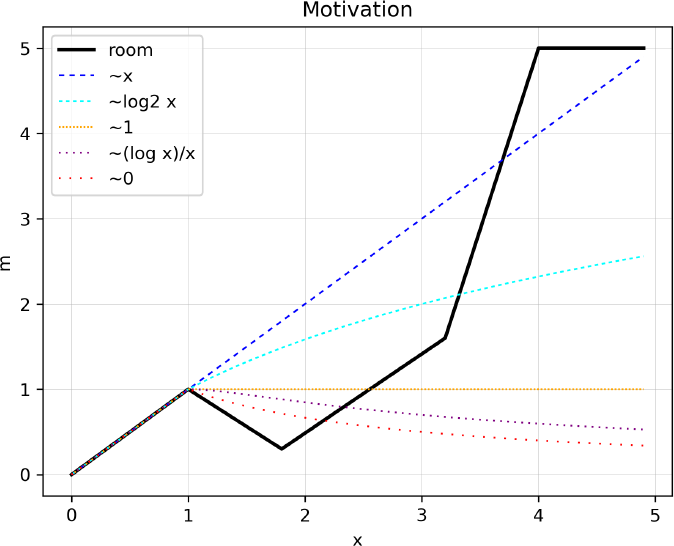
First you introduce an austere room to your client in order to establish the least relevant value 𝑥₁ = 1 . Next you pick up a few representative rooms of rents at 𝑥₂ ≈ 2, …, 𝑥_𝑛−1 ≈ 𝑛 − 1 and ask how much he wishes those rents 𝑥₂, …, 𝑥_𝑛−1 were less by a unit. Namely, 𝑥_𝑖 is the actual rent of room 𝑖 and 𝑚^room(𝑥_𝑖) is how much he wishes the rent were 𝑥_𝑖 − 1. Suppose the rent of the sample room 2 is 𝑥₂ = 1.8 . How strongly the customer wishes it were 𝑥₂ − 𝑥₁ = 1.8 − 1 = 0.8 , compared to 𝑚(𝑥₁) = 1 ? He finds room 2 to be considerably better than room 1 and does not care much about the 0.8 unit difference in rent; the level of motivation to make the rent less by a unit is 𝑚(𝑥₂) = 𝑚(1.8) = 0.3 . Showing two more rooms to the customer and after some conversation you find that the customer’s motivation table should look like

$M^{\mathrm{room}}:=\begin{array}{cccccc}\mathrm{i}& 0& 1& 2& 3& 4\\ x_i& 0& 1& 1.8& 3.2& 4.0\\ m^{\mathrm{room}}\left(x_i\right)& 0& 1& 0.3& 1.6& 5.0\end{array}$

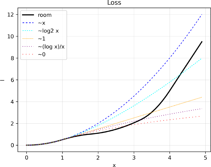
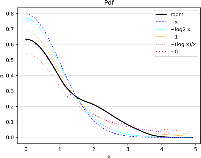
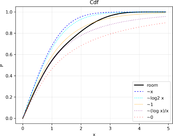
Interpolating linearly the motivation function 𝑚^room becomes as shown in Figure 1 . Figure 2 is the corresponding loss function. The induced pdf and cdf are as in Figure 3 and Figure 4 , respectively. Under the information available as 𝑀^room the pdf 𝑝^room may be considered a distribution of the rent 𝑋 of the room that the customer will choose, conservative in the sense that no extra information is added.

Figure 1
Motivation function 𝑚^room(𝑥).

Figure 2
Loss function ℓ^room(𝑥).

Figure 3
Probability density function 𝑝^room(𝑥).

Figure 4
Cumulative distribution function 𝑃^room(𝑥).

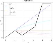
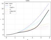
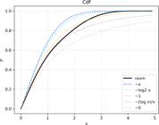
Comparing ℓ^room to ℓ^~X and ℓ^{~log2 x} , the customer seems to be more flexible regarding rent than what the Fechner’s law predicts for 𝑥 ≤ 4 . Since 𝑃^room(2.85) ≈ 0.95 , the rooms of rents over 𝑥 = 2.85 can be omitted from the list of candidates by accepting a 5% error. Perhaps the rooms of rent less than 1.5 or so may also be omitted since the client can afford more expensive rooms. Now you want to take the client to see two candidate rooms, 𝑎 and 𝑏 , for consideration where their rents are 𝑥_𝑎 = 1.8 and 𝑥_𝑏 = 2.5 . The odds that the client prefers 𝑎 over 𝑏 are only 𝑝^room(𝑥_𝑎)/𝑝^room(𝑥_𝑏) ≈ 0.23/0.15 = 1.55 ; it seems worth trying to emphasize comparative advantages of the more expensive room 𝑏 over 𝑎.

4.2 Exam example

Your daughter is going to take an exam and you need to predict the result to be given as a grade 𝑦 from 0 to 100. There are two thresholds: one is that if 𝑦 < 60 she fails the exam; the other is that if 85 < 𝑦 she gets a scholarship. The exam is said to have been calibrated to be normally distributed with mean 𝜇 = 70 and standard deviation 𝜎 = 5 , which is enough information to make a probabilistic prediction if she is to be treated as a random data point from the population of exam takers.

Actually, she has taken a test simulating the exam; her experience should help you make a better prediction. The test consisted of 20 problems and her grade was 76. Set the grade 𝑦’s least signif-icant value to 𝑦₁ ≔ 100/20 = 5 and standardize the grade location to 0 by 𝑥 ≔ (𝑦 − 76)/𝑦₁ = (𝑦 − 76)/5 .

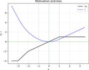
She feels almost sure that she passes the exam. There are various ways to express this, such as setting a barrier to prevent 𝑦 < 60 , but the easiest way would be to set a high enough motivation to avoid low grades as, say,

$M^{\mathrm{exam}-}:=\begin{array}{ccccc}\mathrm{i}& 0& 1& 2& 3\\ y_{\mathit{i}}& 76& 71& 66& 61\\ x_{\mathit{i}}& 0& 1& 2& 3\\ m^{\mathrm{exam}-}\left(x_{\mathit{i}}\right)& 0& 1& 2& 4\end{array}$

She also says that for her all problems in the test were of about the same difficulty. The exam will be more on solving a wide range of problems rather than on solving problems of varying difficulties, which makes you think that it is doubtful that her grade would be normally distributed. You sum up this part of her story as

$M^{\mathrm{exam}+}:=\begin{array}{cccc}\mathrm{i}& 0& 1& 2\\ y_{\mathit{i}}& 76& 81& 86\\ x_{\mathit{i}}& 0& 1& 2\\ m^{\mathrm{exam}+}\left(x_{\mathit{i}}\right)& 0& 1& 1\end{array}$

stating that for 𝑥₁ ≤ 𝑥 or 81 ≤ 𝑦 the cost to solve each extra problem is the same.

Negative and positive parts together specify

$m^{exam}\left(x\right):=\left\{\begin{array}{l}x\le 0\Rightarrow -m^{exam-}\left(-x\right)\\ 0\le x\Rightarrow m^{exam+}\left(x\right)=m^{~1}\left(x\right)\end{array}\right.$

as illustrated in Figure 5 together with ℓ^exam(𝑥).

Figure 5
Motivation 𝑚^exam(𝑥) and loss ℓ^exam(𝑥) functions.

The induced maximum entropy pdf 𝑝^exam turns out to be as in the solid line in Figure 6 the horizontal axis 𝑦 of which is in grades. The vertical lines mark 𝑦 = 70, 76, and 85. The dashed line shows the normal distribution with 𝜇 = 70 and 𝜎 = 5 to which the exam has been calibrated.

Figure 6
Pdf 𝑝^exam(𝑦) and the calibrated normal distribution with 𝜇 = 70 and 𝜎 = 5.

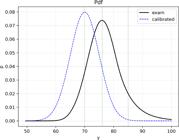
According to 𝑝^calibrated, the chance she gets the scholarship would be one in a thousand, 𝑃^calibrated(85) = 0.001 . However, according to 𝑝^exam, she has a significant 𝑃^exam(85) = 0.101 chance of getting the scholarship which, after her stories, sounds more plausible. Considering that 𝑃(85) = 0.036 for the normal distribution with 𝜇 = 76 and 𝜎 = 5 , the change was brought not only by shifting the mode from 𝜇 = 70 to 𝑦₀ = 76 but also by deflating the left tail of the distribution and inflating the right tail pushing the probability mass to the right.

5 CONCLUSION

A method to specify motivation function 𝑚, which is a short name for standardized negative mar-ginal utility function, has been proposed. The specification of 𝑚 is accomplished by comparing the level of motivation 𝑚(𝑥) against 𝑚(1) = 1 , typically in the form of a table 𝑀 . Integrating 𝑚 produces the loss function ℓ , from which the maximum entropy distribution 𝑝 is induced. Probabilistic inferences are available based on 𝑝 .

The method presented was originally developed to design behavior of machines with limited computational resources. Such applications may need only 𝑚(𝑥) to be computed onboard. Com-putation of ℓ(𝑥) given 𝑚 remains lightweight since it is a table lookup not involving numerical integration of nonlinear functions.

The method helps behavior planning of autonomous machines since the motivation function is secured as a part of the design procedure, but it remains to see how useful the approach can be in producing realistic scenarios when the motivation function is based on qualitative clues at hand.

A possible future research would be to estimate the motivation function given empirical distrib-ution of the status variable.

Acknowledgments

The author is grateful to the Editor for having accepted to review the manuscript prepared with Typst instead of LaTeX, and to the Referees for pointing out deficiencies.

Data availability

All the data investigated are provided in the article.

References

• ALGOM D. 2021. The Weber-Fechner Law - A Misnomer That Persists But That Should Go Away. Psychological Review, 128 https://doi.org/10.1037/rev0000278 .
  » https://doi.org/10.1037/rev0000278
• BOJANIĆ N, FIŠTEŠ A, DOŠENOVIĆ T, ET AL. 2021. Control of the size and compositional distributions in a milling process by using a reverse breakage matrix approach. Hemijska industrija (Chemical Industry), 75 https://www.researchgate.net/publication/349390831%7D .
  » https://www.researchgate.net/publication/349390831%7D
• CONRAD K. 2010. Probability Distributions and Maximum Entropy. https://kconrad.math.uconn.edu/blurbs/analysis/entropypost.pdf .
  » https://kconrad.math.uconn.edu/blurbs/analysis/entropypost.pdf
• KAGIHARA M & YONEDA K. 2009. On Statistical Interpretations of the Semi-Logarithmic Loss Function. https://www.econ.fukuoka-u.ac.jp/researchcenter/workingpapers/WP-2009-003.pdf .
  » https://www.econ.fukuoka-u.ac.jp/researchcenter/workingpapers/WP-2009-003.pdf
• KAREVA I & KAREV G. 2020. 8. Replicator dynamics and the principle of minimal information gain. Modeling Evolution of Heterogenous Populations: Theory and Applications.
• YONEDA K. 2006. A Parallel to the Least Squares for Positive Inverse Problems. Journal of the Operations Research Society of Japan, 49: 279-289 https://orsj.org/wp-content/or-archives50/pdf/e_mag/49-4-279-289.pdf .
  » https://orsj.org/wp-content/or-archives50/pdf/e_mag/49-4-279-289.pdf

• Code availability
  Python programs used to prepare this paper are available upon request.
• Funding
  None.

Publication Dates

• Publication in this collection
  06 Mar 2026
• Date of issue
  2026

History

• Received
  21 July 2025
• Accepted
  28 Oct 2025