Sea-level variability and its impacts on coastal flooding in Baía de Todos os Santos (13oS)

ABSTRACT

This study uses 21 years (2004-2024) of water level measurements carried out by the IBGE’s Brazilian Continuous Monitoring Network (RBMC), in association with the Global Sea Level Observing System (GLOSS), with the aim of quantifying the temporal variability of the water level, identifying long-term trends in mean sea level, and determining the present spatial extent of tidal inundation of the suburban areas of Salvador. Harmonic, statistical, and spectral analyses, complemented by numerical modeling of the hydrodynamics, show that the sea level is rising at a rate of 2.15 mm/yr and the inundation time is increasing. Important seasonal variability is observed, with higher mean sea levels occurring in April and May driven mainly by the wind stress, whose interannual variation also causes alternating interannual MSL trends. The data indicate an increase in the frequency and severity of extreme high sea level events, regularly associated with the passage of subtidal waves that have become higher and more frequent over the years. Numerical simulations showed that subtidal oscillations tend to be amplified inside the estuary, likely increasing the severity of inundation events. A suburban area of 0.497 km² along the bay margin of Salvador, with poor infrastructure, experiences more intense tidal inundation approximately every 4.4 years.

Keywords:
Subtidal oscillations; Sea-level rise; Numerical model; Monitoring

INTRODUCTION

Sea level is a fundamental reference for coastal settlement. It not only limits the seaward expansion of human settlements but also establishes boundaries for different activities, such as navigation, farming, and recreation, and sets a vertical reference for urban planning. The sea level is influenced by periodic and non-periodic oscillations over a large spectrum of frequencies, which for coastal management purposes, range from high-frequency oscillations related to infragravity waves and wave setup (Dodet et al., 2019) to very low frequencies related to interannual climate variability, the nodal tidal cycle, and even secular changes. The interaction of these different oscillations causes considerable complexity in sea-level variability. Extreme high-water levels and coastal inundation occur when various oscillations coincide in phase, elevating the sea level beyond a historical reference elevation used by urban planners.

Underlying these interactions is the present global-mean sea-level rise (GMSLR), an anthropogenic phenomenon that began in the 19th century (Church and White, 2011; Jevrejeva et al., 2009) and is associated with an increase in ocean volume due to both thermal expansion and melting of ice sheets. A linear trend of tide gauge data between 1900 and 2009 indicates the GMSLR increased at a rate of 1.7 mm/yr, but that increases to 3.2 mm/yr if satellite altimetry from 1993-2009 is analyzed (Church and White, 2011). More recently, Hamlington et al. (2024) suggested that a linear fit on long time series can be misleading because it obscures the impact of acceleration in sea-level trends. The global mean acceleration measured by satellite altimetry since 1993 is 0.08 ± 0.06 mm/yr², which caused the sea-level rise rate to increase from 2.1 mm/yr to 4.5 mm/yr in 2023 (Hamlington et al., 2024).

GMSLR is a direct consequence of global warming, which also impacts coastal MSL as the energy stored in the atmosphere causes stronger winds (speed has increased by 0.074% annually since 1940 - Chen, 2025), higher waves (+0.32 cm/yr between 1979 and 2018 - Zheng et al., 2022), and lower atmospheric pressures. The inverted barometer effect accounts for ∼10-30% of sea level rise on the US East Coast between 1950 and 2013 (Piecuch and Ponte, 2015), and these factors together produce larger storm surges. Using a global storm surge numerical model forced with CMIP6 projections, Muis et al. (2023) suggested that half of the 35 defined coastal sectors worldwide will undergo some increase or a significant increase in surge levels by 2050. Storms can impact the mean sea level of distant sites by generating coastal trapped waves (CTWs) of subtidal frequency, which can travel thousands of kilometers from their source region. Freitas et al. (2021) have shown that CTWs generated by storms in Patagonia (65°S) can travel more than 4500 km, inducing small subtidal sea level oscillations in Northeast Brazil (10°S).

However, among the contributors to sea level oscillations, tides are by far the most important, with a spectral power at least three orders of magnitude higher than oscillations excited by other phenomena (Harrison, 2002). The tidal wave is a compound of various harmonics with different amplitudes, frequencies, and phases that cause sea level periodicities to vary from hours to decades. Therefore, understanding the predictable site-specific tidal variability is important for evaluating the probability of inundation at a given time. Tidal oscillations can, however, also be affected by GMSLR, especially in coastal bays and estuaries. Pickering et al. (2012) investigated the effect of a 2 m rise in relative sea level in the North Sea and Irish Sea and suggested that larger tidal ranges may occur over much of the area, with higher rates close to the coast where the spring tidal range could locally increase by up to 35 cm. Inside estuaries, opposing trends can occur depending on whether the topography of the marginal area allows for the growth or reduction of intertidal zones. Oey et al. (2007) showed that the inclusion of intertidal areas in a numerical model of Cook Inlet increased the tidal range by 20%, and tidal ranges in bays and estuaries around the U.K. have apparently increased during the Holocene with an increase in water depth (Hinton, 1995; Shaw et al., 2010).

The Permanent Service for Mean Sea Level (PSMSL) archives data from about 2000 tide gauge stations worldwide, and the Global Sea Level Observing System at the University of Hawaii (GLOSS - UHSLC) provides access to about 600 operational tide gauge stations. Data from 10 stations along the Brazilian coast, covering the period 1947-1967, were analyzed by Mesquita et al. (2013). Although the stations were not operational simultaneously, the data indicated sea-level rise rates between 3 mm/yr and 4 mm/yr. Recently, Efraime et al. (2025) analyzed data from six stations maintained by the Brazilian Institute of Geography and Statistics (IBGE), also part of the GLOSS network, each paired with a Global Navigation Satellite System (GNSS) station. All but one tide gauge station had records spanning more than 17 years, and two stations had records longer than 50 years. Their results indicate a relative sea-level rise rate ranging from 2.2 mm/yr (Ilha Fiscal) to 4.3 mm/yr (Cananéia). Their trend analysis of four tidal harmonic components showed increasing amplitudes of M2 and S2 at the southern stations of Imbituba and Cananéia, at rates up to 0.55 mm/yr. The authors also characterized seasonal and interannual variability, but due to the lack of supplementary climatic time series, no objective causal investigation was performed to explain the observed variability.

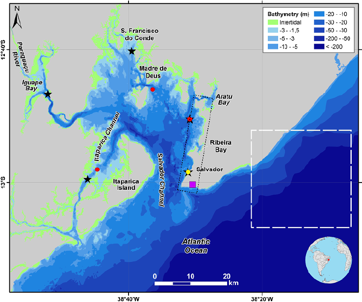
Here, we analyze the sea level signal at the IBGE station in Salvador, at the entrance of Baía de Todos os Santos (BTS - Figure 1) to determine the variability of tidal ranges, extreme high-water levels, and relative MSL rise rates. The BTS is the third largest coastal bay in Brazil (Lessa et al., 2018), where, according to the 2022 IBGE Census (IBGE, 2022), 617,180 people live along the bay shores, often with precarious infrastructure. Therefore, an additional objective of this study is to quantify and evaluate the susceptibility of areas that are currently undergoing the effects of coastal inundation along the suburban areas of the city of Salvador.

Figure 1
Baía de Todos os Santos with location of the IBGE tide gauge (yellow dot), meteorological station (purple square), stations used to validate the simulated tides (red circles), and stations chosen to assess the propagation of the shelf waves (black stars). Dashed white square indicates the location of the Cross-Calibrated Multi-Platform (CCMP) grid element. Rectangle drawn in dotted black line delimits the section shown in Figure 13.

METHODS

STUDY AREA

The BTS is a large (1,223 km²) tectonic, well-mixed, positive estuary (Cirano and Lessa, 2007) centered at 12.83°S and situated behind the narrowest (10 to 15 km wide) stretch of the western South Atlantic continental shelf. The bay has maximum and average depths of 60 m and 9.6 m, respectively, with a main northern inlet (Salvador Channel, Figure 1) 10 km wide and 30 m deep, on average. The tides are semi-diurnal, with form numbers (F=K1+O1/M2+S2) varying from 0.11 on the shelf to 0.06 inside the bay, and explain 97.5% of sea-level variability. The tidal range on the shelf is amplified 1.5 times along the bay, with the main lunar semi-diurnal component (M2) growing from 0.67 m to 1.06 m 60 km upstream (Cirano and Lessa, 2007). The tides are asymmetric inside the bay, favoring a faster ebbing tide, and this asymmetry is increased landward.

The BTS catchment area is 61,110 km² (Lima and Lessa, 2001), with 90.5% of this area corresponding to the drainage of the Paraguaçu River, which reaches the bay in its western extreme (Figure 1). The remainder of the catchment includes the rivers Jaguaripe (3.6%), Subaé (1.1%), and several small peripheral creeks (3.2%) (Lima and Lessa, 2001). The rainfall seasonality in the upper catchment is out-of-phase with that on the coast. The highest Paraguaçu river discharges occur between November and March, the dry season on the coast. The Paraguaçu River accounts for 76% (69.5 m³/s) of the total mean annual fluvial discharge that reaches the bay (Genz and Lessa, 2015). This flux corresponds to 0.4% of the equinoctial spring-tidal prism of about 3.1×10⁹ m³ (Cirano and Lessa, 2007).

The wind blows from E-ENE in the summer and from ESE-SE in the winter, with a maximum mean speed of ~10 m/s. ESE-ENE winds drive frequent coastal upwelling between September and March, which are longer lasting and more intense in front of the BTS (Santos et al., 2014; Thévenin et al., 2019). An 11-year wave time series obtained by an ADCP on the continental shelf at a depth of 32 m (12.6°S) indicates that east waves prevail in the spring and summer with significant heights between 1 m and 2 m and periods between 6 s and 8 s. In autumn and winter, SE waves are more frequent, with significant heights between 2 m and 3 m and periods between 6 s and 10 s (Pereira et al., under review). The highest wave height and period were 4 m and 17 s.

DATA ANALYSIS AND PROCESSING

Sea-level data were recorded by the IBGE tidal station located at the Coast Guard pier about 150 m from the shore, where a GNSS station is located. The tidal station was instrumented with an acoustic Aquatrack 4100 sensor with a recording interval of 6 min between November 2004 and December 2008. In April 2008 the acoustic sensor was replaced by a sonic Vegapuls 62 radar and a Sutron Encoder SDR with recording intervals of 1 min and 5 min, respectively (IBGE, 2022). This station is part of the GLOSS network (station number 334) and hourly data are made available both by the IBGE Permanent Geodetic Tide Gauge Network (RMPG) and by the University of Hawaii Sea Level Center (UHSLC) (Caldwell et al., 2015).

Research-quality data from UHSLC were obtained for the period 01/01/2005 to 31/12/2018, complemented by a Fast-Release time series to December 2024 (Caldwell et al. 2015). The time series accessible at IBGE extends from January 2004 to December 2023. When comparing the UHSLC and IBGE time series, small differences in weekly-to-monthly MSL were detected. This was especially the case with the Fast-Release data, which caused phase angles of semi-diurnal constituents to deviate a few degrees from preceding values. With the aid of harmonically reconstructed time series, careful adjustments were made between the two data sets in order to produce a complete 21-year record spanning from 2004 to 2024.

The data were interpolated to a 10-minute interval with a spline function in order to make tidal asymmetry calculations possible, and were referenced to the local Navy Hydrographic Center reduction level (RL), which is used as a reference level for nautical charts and tide tables. Locally, the RL is 2.286 m below MSL and 0.122 m below the tide staff zero, which is the reference for the GLOSS water level data.

The sea level signal was band-pass filtered between cut-off frequencies of 1/53 hours and 1/720 hours (~1 month) to eliminate both subtidal and seasonal oscillations, respectively. The cut-off periods correspond to the inertial period at this latitude (53 hours) and the longest subtidal wave period identified by previous studies (Freitas et al., 2021). Height and period of subtidal oscillations were calculated using the upward zero-crossing method.

Trend analysis of the time series was performed with Mann-Kendall and Sen’s slope tests. The former statistically tests whether there is an upward or downward monotonic trend over time, whereas the latter calculates the magnitude and direction of the identified trend. The trends were statistically tested considering a 95% confidence interval.

Harmonic analysis was performed with the T_TIDE package (Pawlowicz et al., 2002) to investigate the variability of diurnal and semi-diurnal components. Because of T_TIDE difficulties in dealing with very long time series, the extraction of the harmonic components for the 21-year time series was performed with the U_tide Matlab package (Codiga, 2011).

Calculations of tidal asymmetry were executed both through the rise/fall ratio of each tidal cycle (values higher than 1 indicate faster falling tides) and through the phase and amplitude relationships between M2 and M4 tidal components, according to M4/M2 and 2(M4-M2), respectively. Higher ratios are associated with larger distortion of the tidal wave, whereas phase differences between 0° and 180° (180° and 360°) indicate faster rising (falling) tides (Friedrichs and Aubrey,1988). Given the (small) range inequality between successive tidal cycles, tidal ranges were calculated between low and high tide (TRLH) and between high and low tide (TRHL). Water level duration curves were calculated annually using elevation classes between 0.4 m and 3.89 m with increments of 0.1 m. The curves were normalized at 2.5% intervals using a piecewise cubic interpolator (PCHIP). The statistics for spring and neap tide ranges considered the range of 5 cycles centered at the highest and lowest tidal range, respectively, within the spring-neap cycles.

Atmospheric pressure data were obtained from a station maintained by the Brazilian National Meteorological Institute (INMET - https://portal.inmet.gov.br) located close to the BTS entrance from 2005 to 2024 (Figure 1). The hourly data were subjected to quality-control analysis, with spurious data identified as values higher (or lower) than the 6-hour mean (centered at the time of interest) plus (minus) 2 times the standard deviation (Emery and Thomson, 2004).

Wind data were downloaded from the Cross-Calibrated Multi-Platform (CCMP - https://www.remss.com), a 6-hour interval combination of ocean surface 10 m wind retrievals from multiple types of satellite microwave sensors and a background field from reanalysis, with a spatial resolution of 0.25°. A time series of north (vN) and east (vE) velocities was extracted from a grid element closest to shore centered at 13.125°S and 38.125°W (Figure 1). This grid element is the closest to METAR (SBSV) meteorological station (useful data from 2009 onwards) and to the SiMCosta BA1 buoy (data from 2019 to present), which were used to ground-truth the CCMP data set. A preference for CCMP data was given because it covers the whole tidal time series and because of existing biases at the METAR and SiMCosta records caused by the terrain; the former underestimates S and SE winds, while the latter underestimates E and NE winds. The alongshore wind component, responsible for the shore-normal Ekman transport, was calculated according to V = -vE sinq + vN cosq, in which q is the coastline orientation (−40° in the immediate region). Both the wind speed and atmospheric pressure were low-pass filtered using a cut-off period of 53 hours.

On 8 February 2024 the region was subjected to extensive tidal flooding, when the crest of a subtidal wave coincided with an equinox-spring tide at a time close to the lunar perigee. Numerous events of flooding and beach erosion were reported by the media in Salvador and other 30 coastal municipalities, including those located inside the BTS. The tide table published by the Navy Hydrographic Center (https://www.marinha.mil.br/chm/tabuas-de-mare) predicted a maximum spring high-tide level of 2.8 m (relative to RL) for February 8, which will henceforth be taken as a reference elevation for coastal inundation.

A high-resolution LIDAR topography of the metropolitan area of Salvador (SEFAZ, 2017), carried out between 2016 and 2017 with a spatial resolution of 1:1000, was used to identify areas between the BTS entrance and Baía de Aratu (Figure 1) that are prone to inundation by high tides. The LIDAR vertical datum is the MSL at Imbituba Harbor (IMB datum - a national vertical datum established by IBGE), which is 0.86 m above the local RL. Elevation classes defined by the tidal datum Mean Water Level (MWL), Mean High Water Neap (MHWN), Mean High Water (MHW), Mean High Water Spring (MHWS), and Maximum High-water Level (MHL) were drawn along the shoreline.

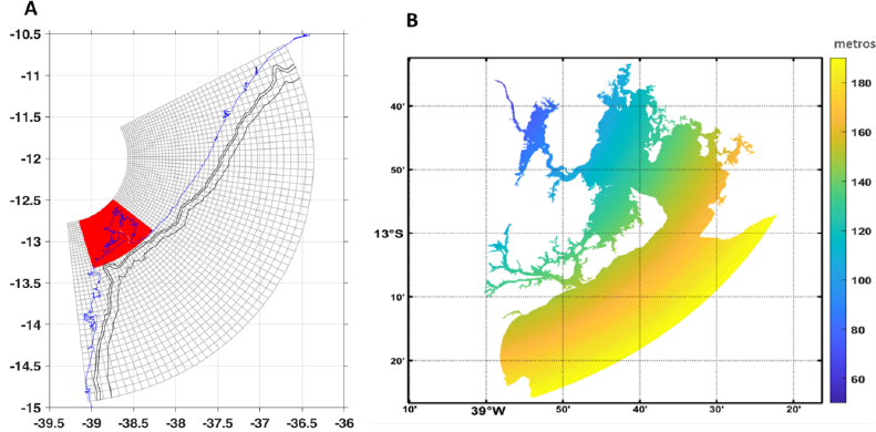
A numerical simulation of the bay hydrodynamics was used to assess the propagation of subtidal waves inside the BTS. A Regional Ocean Modeling System (ROMS) was implemented for the region with two nested meshes (Figure 2a) (Franklin et al., 2026). The higher-resolution mesh covered the whole bay and neighboring shelf with grid spacing varying between 200 m and 50 m (Figure 2b). Hourly solutions between 2008 and 2021 were forced using global winds from CFSR, boundary conditions from GLORYS-Mercator, and initial conditions from HYCOM. As additional boundary conditions, daily-mean discharges of 43 rivers, 15 of which discharge into the BTS, were incorporated. Data from gauged rivers were obtained from the Brazilian National Water Agency (ANA) website. For smaller, unmonitored rivers, discharge was estimated using area-discharge relationships with the nearest gauged river.

Figure 2
The domain of the two nested numerical grids used in ROMS (A) and the variable spatial resolution of the higher-resolution grid (B).

Tides were imposed at the model open boundary through the main harmonic components (M2, S2, N2, K2, K1, O1, P1, Q1) from TPXO 8.0 (Egbert and Erofeeva, 2002), with a spatial resolution of 1/12th degrees. The grid bathymetry was obtained from a blend of ETOPO with high-resolution nautical charts produced by the Brazilian Navy (https://www.marinha.mil.br/chm/dados-do-segnav/cartas-raster), whose scales varied from 1:350,000 on the continental margin to 1:8,000 inside the bay.

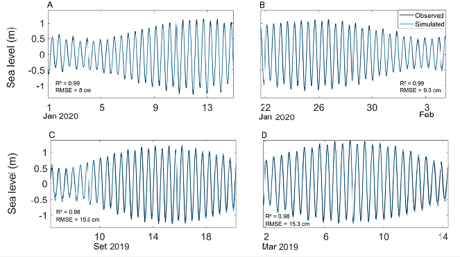
Five sites were chosen to validate the model results (black stars in Figure 1): one coincident with the IBGE tidal station and four others in more interior positions where tidal records exist. A comparison of the observed and simulated time series is shown in Figure 3. Correlation coefficients are higher than 0.98 for all stations, with RMSE of 0.08 m in Salvador, 0.09 m in Aratu Channel, 0.16 m in Madre de Deus, and 0.15 m in Itaparica Channel. In Salvador and Aratu Channel the error corresponds to 4% of the spring tidal range, whereas in Madre de Deus and Itaparica Channel it corresponds to 6% of the spring tidal range of the compared time series. Higher errors at the two inner stations are ascribed to the inability of the numerical grid to reproduce the complex bathymetry around Madre de Deus and to the low-resolution nautical chart (1:60,000) that covers Itaparica Channel (Franklin et al., 2026). A complete validation of the numerical model can be found in Franklin et al. (2026).

Figure 3
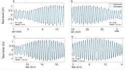
Observed (black) and simulated (blue) sea level variation at 4 sites within the BTS. Correlation indices (R) and the root-mean-square error (RMSE) are indicated for each site. A) IBGE station, B) Aratu, C) Madre de Deus, and D) Matarandiba.

To investigate the propagation of subtidal oscillations, five sites were chosen in the model grid (red dots in Figure 1) which are representative of the innermost urban centers around the bay. We used the time series of 2020 for this analysis, a year with a higher frequency of large subtidal oscillations. The elevation difference between the simulated high tide and the high tide obtained from the reconstituted tidal oscillations provided a measure of the coastal flooding.

RESULTS

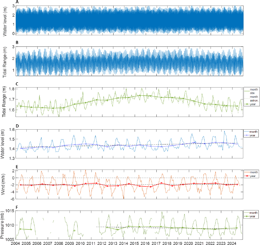
The complete water level time series is shown in Figure 4a. Minimum, maximum, and mean water levels were −0.11 m (September 2015), 3.02 m (April 2024), and 1.43 ± 0.62 m, respectively (Table 1). MHWS and MHWN were 2.58 ± 0.14 m and 1.94 ± 0.12 m, respectively, whereas MLWS and MLWN were 0.30 ± 0.13 m and 0.96 ± 0.10 m, respectively (Table 1).

Figure 4
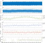
Time series of the tides at IBGE station (A), tidal range of each tidal cycle (B), monthly- and yearly-mean tidal ranges (C), monthly- and yearly-mean sea levels (D), monthly- and yearly-mean alongshore wind speeds from CCMP (E), and monthly- and yearly-mean air pressure from INMET - Salvador station (F). Months or years with less than 80% of valid data were not included.

Table 1
Characteristic tidal range values for the Salvador Harbor tidal station in relation to the local hydrographic datum (RL) and Imbituba datum (IMB), which is the national vertical datum.

Datum	Elevation (m) RL	Elevation (m) IMB
HWL	3.02	2.16
MHWS	2.58 ± 0.14	1.72
MHW	2.28 ± 0.27	1.42
MHWN	1.94 ± 0.12	1.08
MWL	1.43 ± 0.62	0
MLWN	0.96 ± 0.10
MLW	0.60 ± 0.27
MLWS	0.30 ± 0.13
LWL	-0.11
Tidal Ranges (m)
Mean tidal range	1.67 m ± 0.52
	Spring	Neap
Mean range	2.28 ± 0.06	0.98 ± 0.08
Max range	2.88	1.55
Min range	1.65	0.44

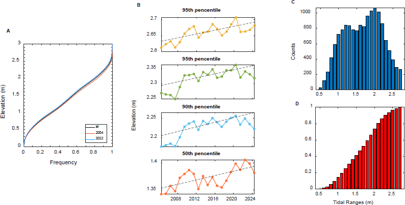
The water-level duration curve (Figure 5a) shows that the water level stays between 0.88 m and 1.9 m for 50% of the time, with a median value of 1.37 m. However, these frequencies exhibited an increasing trend over the 21 years, as indicated by the curves for 2004 and 2022, whose median values are 1.35 m and 1.41 m, respectively. The trend is more evident when the annual variation of higher percentiles is considered. Figure 5b shows the trends progressively increase from 2 mm/yr to 3 mm/yr between the 50th and 99th percentiles, accounting for respective total increases of 4.2 cm and 6.3 cm in their elevation over 21 years. Figure 5b also shows a 4-year modulation that becomes more conspicuous at the higher percentiles, reaching an amplitude of 5 cm at the 99th percentile.

Figure 5
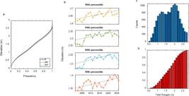
Water level duration curve for 2004, 2020, and a mean curve for the 21 years of data (A). The variation of key percentiles of the sea-level cumulative-frequency distribution (B), the frequency distribution of tidal ranges (C), and its cumulative-frequency distribution (D).

Seasonal variations in the water level are well established, with lower sea levels in spring and summer and higher sea levels in autumn and winter (Figure 4d). The seasonal amplitudes fluctuate between 14 cm and 18 cm. This seasonality is well explained by variations in the wind direction (Figure 4e), with a correlation coefficient of 0.61. During the spring and summer, the wind blows southward (negative values), causing an offshore Ekman transport that lowers MSL. Conversely, winds blowing northward in autumn and winter push water against the coast and elevate the MSL. The correlation coefficient decreases significantly, to 0.29, when the mean-annual MSL and wind are analyzed. Monthly-mean air pressure is not correlated with MSL (Figure 4f). However, mean-annual values show a negative correlation of −0.69, indicating that the inverse barometer effect plays a role in the interannual MSL variability.

The annual MSL between 2004 and 2021 rose at a linear rate of 2.15 mm/yr, as indicated by the dashed black line in Figure 4d, or a rate of 1.85 mm/yr if monthly means are considered. The mean-annual values indicate important interannual oscillations. MSL rose between 2004 and 2010, decreased between 2010 and 2017, and rose again through 2024, with in linear trends of 7.82 mm/yr, −3.71 mm/yr, and 4.80 mm/yr, respectively, although the last two are not statistically significant. Wind velocity showed a very small, positive but not statistically significant trend of 0.01 m/s.yr, and air pressure presented a negative, but also not statistically significant, trend of −0.059 mb/yr. Both trends would contribute to a sea-level rise.

The mean tidal range was 1.67 m ± 0.52 m, varying from a minimum of 0.44 m (October 2004) to a maximum of 2.88 m (September 2019) (Figure 4b). The mean, minimum, and maximum spring tidal ranges were 2.28 ± 0.06 m, 1.65 m, and 2.88 m, whereas the mean neap tidal range was 0.98 ± 0.08 m, with a maximum of 1.55 m and a minimum of 0.44 m (Table 1). The frequency distribution of tidal ranges is bimodal (Figure 5c), with the most frequent ranges being 1.2 m and 2 m, which correspond to the 25th and 75th percentiles (Figure 5d). Mean spring and neap tide ranges are 2.31 m ± 0.19 m and 0.96 m ± 0.16 m, respectively. Differences between low-to-high tide range and high-to-low tide range can reach 0.4 m either way (Figure 6), but are modulated by fortnightly, monthly, semi-annual, and annual cycles. Larger high-to-low tide ranges (negative values in Figure 6) tend to occur at high spring tides, an additional forcing agent to the documented ebb dominance of tidal currents (Cirano and Lessa, 2007).

Figure 6
Variation of the difference between low-to-high tide and high-to-low tide ranges for the year 2018. In gray the differences for each tidal cycle and in black the low-pass filtered signal with a cut-off period of 15 days. In red the range of each tidal cycle, highlighting spring-neap cycles.

The influence of equinox tides is clearly seen in Figure 4 b and c, with two peaks of tidal range occurring every year. The ranges show a long-period oscillation associated with the nodal cycle (Figure 4c), with the annual-mean tidal range increasing by 0.12 m between a minimum in 2007 and a maximum in 2015. The Sen’s slope estimate on themean-annual data indicates the tidal ranges are increasing by 1.2 mm/yr, which amounts to a 4 cm increase in 21 years.

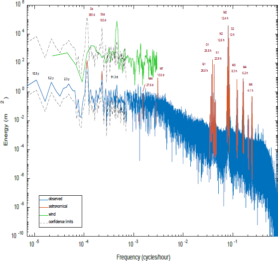
Spectral analysis of the time series (Figure 7) shows the importance of overtides (M6, M4 and M3), semi-diurnal (M2, S2 and N2), and diurnal (K1, O1 and Q1) tides in the sea level variability. The red line in Figure 7 highlights the spectral peaks associated with the reconstituted astronomical tide, which explain 99.5% of the total water level variance. Important non-astronomical periodicity occurs at periods of 91.3 days, 2.3 years, 5.2 years, and 10.5 years. The 91.3-day cycle is associated with the wind, which presents a distinct energy peak at the same frequency.

Figure 7
Power spectrum of the observed and reconstituted astronomical tide at Salvador harbor based on 21 years of records. Main harmonic components are identified. The wind spectral density shows some correspondence with the sea level at the 91.3-day cycle.

The harmonic analysis of the whole time series resolved 68 constituents, and the most important ones for each periodicity class are shown in Table 2. The reconstituted astronomical tide accounted for 99.6% of the measured water level variance. On a monthly basis, it explained between 98% and 100% of the measured water level variance, with the lowest and highest monthly average values occurring around the solstices and equinoxes, respectively.

Table 2
Amplitude and phases (relative to local time) of important tidal harmonic constituents resolved from a 21-year record from Salvador Harbor.

Constituent	Amplitude (cm)	Phase (°)	Constituent	Amplitude (cm)	Phase (°)
SA	4.79	121	MU2	3.24	124
SSA	2.11	85	N2	14.60	109
MSM	0.14	202	M2	79.10	112
MM	0.40	359	L2	2.34	99.6
MSF	0.24	73.3	S2	31.20	127
MF	1.40	350	K2	8.94	121
Q1	1.76	94.8	M3	1.11	125
O1	6.36	124	MN4	0.39	185
P1	1.38	199	M4	1.19	269
K1	3.89	211	MS4	0.93	16.8
2N2	2.22	108	M6	0.30	353
NU2	2.62	104

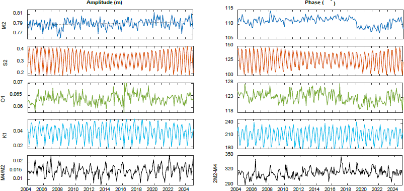
Eighteen semi-diurnal and twenty-two diurnal constituents account for 82% and 9%, respectively, of the total astronomical tidal amplitude. The overall tidal form-number is 0.09, but it varied regularly with the seasons, associated with the sun’s latitudinal excursion. The smallest form-numbers, as low as 0.06, occurred during the autumnal equinox, whereas the highest values occurred during the winter solstices, reaching up to 0.12 (not shown). This seasonal variability is forced by the out-of-phase oscillations of the semi-diurnal constituents and K1 (Figure 8); i.e., maximum semi-diurnal amplitudes coincide with minimum K1 amplitudes. The monthly amplitudes of the four main tidal constituents oscillated between 0.72 m and 0.85 m for M2, 0.26 m and 0.43 m for S2, 0.04 m and 0.09 m for O1, and 0.01 m and 0.07 m for K1 (Figure 8). A statistically significant linear trend occurs only for the M2 amplitude, which increased at a small rate of 3.2 × 10^-2 cm/yr over 21 years.

Figure 8
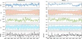
Monthly variability of amplitude and phases of the main semi-diurnal and diurnal constituents, and the measures of intensity (amplitude ratio of M4/M2) and sense (phase angle difference 2M2-M4) of tidal distortion. Dashed line in M2 amplitude indicates the only statistically significant linear trend.

Monthly M2 phase angles varied by up to 7° over 21 years, with a minimum of 107° in December 2021 and a maximum of 114° in March 2008 (Figure 8). The M2 phase angle underwent a reduction of about 3° after 2019, but this should be considered an artifact because it coincides with the transition between UHSLC and IBGE time series. Similar variability is observed in the phase angles of the other constituents in Figure 8. The amplitudes of S2 and K1 show distinct seasonal cycles, varying by up to 0.2 m and 0.03 m, respectively, while their phase angles vary by almost 50°.

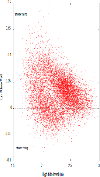
The monthly M4/M2 ratio varied between 0.008 and 0.03, with annual maximum occurring mostly at the summer solstices (Figure 8). The monthly mean amplitude of M2 tends to be negatively correlated with M4 amplitude. The M4 and M2 phase angle difference oscillated around two modal values, 310° and 200°, the latter coinciding with the smallest M4/M2 ratios in the spring equinoxes. These phase-angle differences are close to 270° which is associated with the maximum tidal distortion favoring shorter falling tides. In fact, the mean, median, maximum, and minimum values of the rising/falling time ratio are 1.03±0.06, 1.02, 1.39, and 0.79, respectively. Figure 9 shows the natural logarithm of the rising/falling time ratio against the high-tide level. A logarithmic representation is chosen because it produces a proportional graphical distribution of ratios around zero, with positive (negative) ratios indicating shorter falling (rising) tides. It is observed that positive log values are more numerous, and the degree of asymmetry is modulated by the tide range, with larger asymmetries occurring during neap tides and smaller asymmetries during spring tides. The tidal oscillations tend to be more symmetrical at very large spring tides.

Figure 9
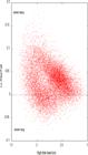
Variation of the natural logarithm of the rising/falling time ratio against the high-tide level. Positive (negative) log values indicate shorter falling (rising) tide.

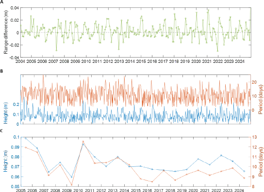
The monthly-mean ranges of the reconstituted astronomical tides differ by a maximum of 4 cm from those of the observed records, with the reconstituted tidal ranges averaging 3.5 cm less than those observed. Figure 10a shows the variability of this monthly difference over the 21 years, with seasonal cycles of larger positive differences occurring in the austral summer. The range of the subtidal sea-level oscillations (Figure 10b) reached up to 0.28 m, with periods varying between 2.2 days and 25.8 days. Wave height and period are positively correlated, with a correlation coefficient of 0.69 for the complete series and 0.88 for the annual mean. Mean subtidal wave height and period are 7.4 cm and 9.7 days, respectively. The yearly means in Figure 10c suggest a linear trend of 2.9 × 10⁻⁴ cm/yr for wave height and −0.1 days/yr for wave period, although these trends are not statistically significant. This may indicate that subtidal wave period is decreasing while wave height is increasing.

Figure 10
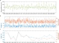
A) Variability of the monthly-mean tidal range difference between the observed and the reconstituted astronomical tide, B) Variability of the height and period of subtidal oscillations and their annual-mean values (C).

As indicated by the water level frequency distribution in Figure 5a, the severity of coastal inundation has increased over the years. Figure 11a shows the monthly and yearly total number of hours with water level above 2.8 m (the assumed threshold for coastal inundation), calculated both with the reconstituted astronomical tide and the observed tide. The threshold is exceeded seasonally around the equinoctial tides, especially during the austral autumn equinox, with a maximum of 14 hours of inundation in March 2020. The predicted inundation period tends to be smaller than the observed one, especially in the last 10 years. The observed total yearly hours were always higher than predicted, and more than doubled between 2006 (14 hours) and 2024 (32 hours). A cycle with approximately four years is clearly established in the duration of inundation and in the maximum elevation of the mean spring equinoctial tides (Figure 11b), which also shows an increasing linear trend at a mean rate of 0.4 cm/yr, or a total of 8 cm in 21 years.

Figure 11
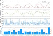
A) Total monthly and yearly hours with water level equal to or higher than 2.8 m considering the observed records and the reconstituted astronomical tide. B) Maximum elevation of the observed mean spring equinoctial tides and the potential elevation if they coincided with the crest of the subtidal wave that occurred nearest to them. C) Elevation difference between the maximum surge elevation and the mean high water of spring tide cycles equal to or above 2.45 m (90th percentile of the distribution). Positive values indicate potentially higher spring high tides. Zero values indicate spring tides were coincident with the maximum surge elevation (equals the bar graph). D) Number of storm surge events coincident with spring tidal cycles equal to or above 2.45 m and total number of subtidal waves per year.

Subtidal sea level oscillations have become progressively more important as a driver for coastal inundation, as the difference between the predicted and observed extent of inundation indicates. The number of subtidal oscillations increased from 31 to 44 between 2005 and 2009, decreased to 29 in 2010, and then established a rising trend modulated by 3- to 4-year oscillations (Figure 11d). Very few of these waves occurred concurrently with spring tides reaching water levels above 2.45 m (very-high spring tides), which is the 90th percentile of the cumulative water level distribution (as shown in Figure 5). Figure 11c shows the elevation difference between the crest of the subtidal wave that occurred within a 14-day window centered on the very high spring tide and the mean high-water level of that spring tide. Differences smaller than 1 cm are associated with spring tides that coincide with the crest of the subtidal waves; the annual number of such coincidences is given by the bars in Figure 11d. An average of 4 subtidal waves per year, or about 10% of the total number of subtidal waves identified per year (Figure 11d), coincided with very high spring tides. The elevation difference indicates that the very high tide levels could have been up to 16 cm higher if such a coincidence had occurred, raising the maximum elevation of several of the mean spring equinoctial tides, as shown in Figure 11b.

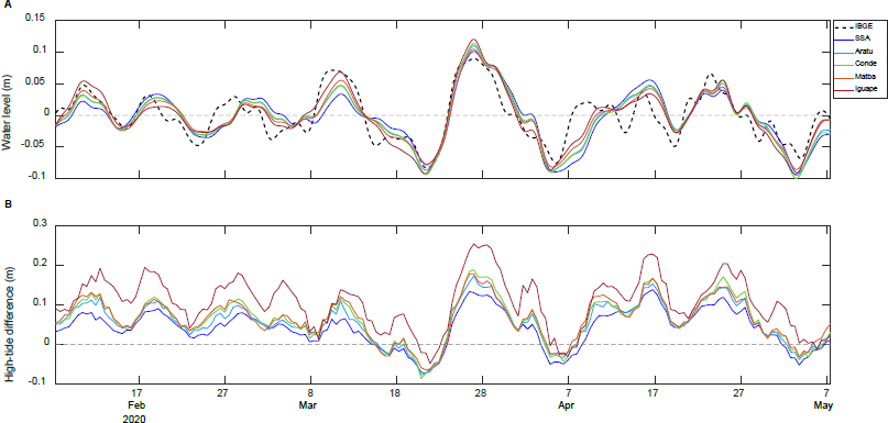
The effects of water level superelevation caused by subtidal oscillations appear to be exacerbated farther inland from the tide gauge station. Using the time series obtained from the numerical model at five stations around the bay (Figure 1), it is observed that the amplitude of the subtidal oscillations becomes larger farther inland. Figure 12a shows the band-pass (53 h to 30 days) water level variation between February and May 2020, with seven subtidal waves; the largest amplitude of 21 cm occurred in late March. The dashed black line shows the observed oscillations at the IBGE station. Four of those waves grew in amplitude landward, including the ones with the largest amplitudes in March. Differences between the simulated high-tide elevation and the predicted high-tide elevation, based on harmonic analysis of the simulation results, show that high-water superelevation increases farther inland (positive differences), reaching a maximum at Maragojipe, where the high-tide level was 28 cm higher than predicted on March 28 (Figure 12b). Negative differences occur occasionally during wave troughs.

Figure 12
A) Band-pass filtered water levels at the IBGE tidal station and simulation results from 5 different sites. Simulation results from site SSA correspond to the observed IBGE time series. B) High-tide level difference between the simulated time series and the reconstituted astronomical high tide based on harmonic analysis of the simulation results for each site inside the BTS.

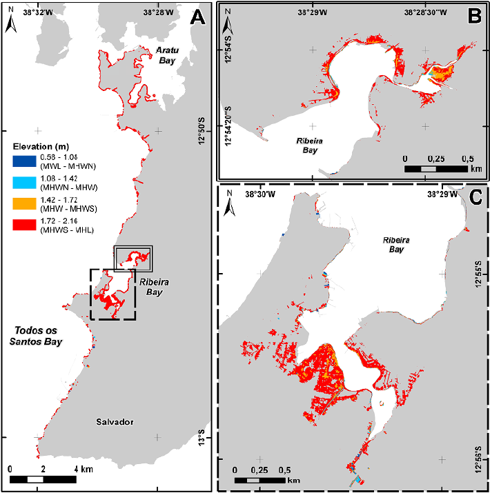
The LIDAR data indicate that coastal inundation of urbanized areas occurs mostly as a narrow band along the shoreline (Figure 13a), covering an area of 0.497 km² with elevations above MWL. The large majority (84.6 %) of the inundation occurs in areas above 1.72 m in elevation, or above MHWS (Table 3), as clearly indicated by the large expanses of this elevation class in Figure 13. About three-quarters of all inundation areas (0.375 km²) are located on the margins of Baía da Ribeira (Figure 13 b and c), where 79% of the whole area between MHWS and MHL is located. Again, inside this small bay the highest elevation class prevails.

Table 3
Distribution of the inundation area between tidal datum above MWL

Elevation	Datum	Whole Area		Baía da Ribeira
(m)		(m2)	(%)	(m2)	(%)
0 - 1.08	MWL - MHWN	37,632	7.6	8,920	2.4
1.08 - 1.42	MHWN - MHW	3,176	0.6	3,003	0.8
1.42 - 1.72	MHW - MHWS	35,713	7.2	31,372	8.4
1.72 - 2.16	MHWS - MHL	419,992	84.6	332,030	88.5

Figure 13
Urbanized areas undergoing inundation along the Salvador bay shores at different elevation classes (A). Detail of Baía da Ribeira southern and northern segments. Ground elevation from LIDAR measurements (SEFAZ, 2017).

DISCUSSION

The astronomical tide in Salvador accounted for at least 98% of the monthly water level variance and explained 99.6% of the variance of the entire time series, implying a very small influence of subtidal sea-level oscillations. In fact, subtidal oscillations larger than 0.2 m in height, which correspond to 8% of the mean tidal range, account for only 1% of the subtidal oscillations in the record. The subtidal oscillations in Salvador are almost 10 times smaller than those reported in southern Brazil. Vianna et al. (2020) report low-frequency waves of 1 m in Imbé (RS - 30°S), Truccolo et al. (2006) report subtidal oscillations with ranges of up to 0.9 m in São Francisco do Sul (26.25°S), and Schettini et al. (2019) report a maximum range of 0.85 m in Santos (24°S). A study on meteorological tides along the Atlantic coast of South America by Melo Filho (2017) shows a strong south-to-north reduction in the contribution of subtidal oscillations to the water level variance between Rio Grande (32°S) and Fortaleza (3.6°S), from an astonishing 76% in the former to 0.2% in the latter. This trend is a consequence of several factors: reduced wind and atmospheric pressure disturbances toward lower latitudes, increasing tidal amplitude away from an amphidromic point near 32°S, and energy loss as subtidal waves propagate away from subtropical latitudes where cyclogenesis is more frequent. Freitas et al. (2021) show that shelf-wave amplitude is damped north of 22°S because of increasing morphological complexity of the continental shelf, but especially north of 15°S where the shelf narrows considerably.

Coastal flooding becomes sporadic where subtidal oscillations constitute only a fraction of the tidal amplitude, such as in northern and northeastern Brazil. At these sites, coastal flooding tends to occur during equinoctial spring tides, limited to periods around high tide. This is because large tidal ranges, or swift changes in water levels, reduce the frequency that water levels remain above inundation thresholds. Sweet and Park (2014) showed that San Francisco (37°N), with a mean greater diurnal range of 1.9 m, is up to five times less likely to experience coastal inundation than Galveston (29°N), where the mean greater diurnal range is 0.62 m.

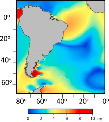
Salvador does not show an increase in the number of inundation events over the years, with a maximum of about 15 events roughly every four years. This ~4-year cycle is related to the combination of the monthly tidal constituent MM and the semi-annual solar constituent SSA, the former associated with the perigee-apogee cycle and the latter with the latitudinal transit of the sun. As the mean longitude of perigee crosses the equator, lunar perigean, lunar declination, and solar equinox act together to reinforce spring tides. As perigee precesses through its 8.85-year cycle, it passes each equinox twice, generating a 4.4-year periodicity (Ray and Merrifield, 2019). This tidal modulation, which can greatly influence coastal inundation, is greatest along the northeastern Brazilian coast, with amplitudes varying between 4 and 6 cm, but is almost nonexistent along the coast of Rio de Janeiro according to Ray and Merrifield (2019) (Figure 14).

Figure 14
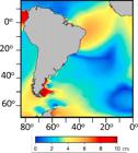
Amplitude of the 4.4-year modulation of extreme tidal high water (modified from Ray and Merrifield, 2019).

Although the number of inundation events per year has not increased, the duration of submergence at the peak of the 4-year cycle increased by 20 hours per year between 2006 and 2020/2024. This is explained by a higher number of subtidal oscillations occurring at this latitude, especially in those years when the astronomical tidal forcing was at its maximum. Moreover, there appears to be an increasing trend in the amplitude of subtidal oscillations. More frequent subtidal oscillations can be ascribed to a positive trend in storminess in the southwestern South Atlantic. De Cai Conrado et al. (2024) showed a positive, statistically significant storminess trend between 20°S and 35°S in the 1900-2010 reanalysis data from ERA20C, a trend that is also observed in the more recent 1970-2010 period. In line with these results, Gramcianinov et al. (2023a, 2023b) found an increase in significant wave height and wave period using ERA5 reanalysis data between 1993 and 2021 in the same region. It is also possible that the local action of storm winds in supra-inertial frequencies may cause a storm surge that coincides with the crest of a subtidal oscillation. This potential synergy has not been investigated and is an avenue for further studies.

Coastal inundation of the suburban area of Salvador occurs along the margins of Baía da Ribeira, on pre-existing mangrove areas that were extensively filled between the 1950s and 1980s, the removal of which reduced the bay area by 43% (Franklin and Lessa, 2011). This area covers 0.375 km² of neighborhoods with a population of ~109,000 (IBGE Census 2022), and a population density of 372 inhabitants/km². It has already been mapped as a suburban area with the highest risk of inundation by rising sea levels (Nicolodi and Petermann, 2010). The mapped areas are likely larger in the northern sections due to the landward tidal amplification in the bay; i.e., the reference elevation from Salvador used in the analysis underestimates the tidal flooding in more interior parts of the bay. Because high tide levels impede the drainage of pluvial waters, and given that extraordinary high tide levels are commonly associated with storm surges, the potential extent of tidal inundation is likely worsened by compound flooding, i.e., the damming of pluvial waters. For instance, it is suggested that the synergy between these phenomena in Macau increases the inundated area by 19% and causes the underground drainage to back up for 1.4 km inland from the coastal boundary (Gao et al., 2023).

The increase in the amplitude of subtidal waves as they propagate into the BTS may exacerbate coastal flooding scenarios in low-lying areas farther inland. The increase in high-tide elevation would be up to 5 cm higher than that experienced in Salvador at all of the sites investigated (Figure 12), except for the innermost site in Iguape Bay, where the superelevation would be almost 15 cm higher than that in Salvador. Similar behavior is reported for large convergent estuaries where flow impedance at the inlet is not significant and tides are amplified upstream (Lyddon et al., 2019; Spicer et al., 2019), such as the BTS. Spicer et al. (2019) show that in inland estuarine regions where river discharge becomes progressively more important, high-tide superelevation is intensified due to damming of the river flow. This phenomenon would help to explain the higher high-tide elevation differences in Maragojipe, where the Paraguaçu River exits into the bay.

The amplitude of the M2 tidal constituent increased at a rate of 3.2 × 10^-2 cm/yr, totaling 0.6 cm over the observation period. This is consistent with the almost null trend found by Efraime et al. (2025) in Salvador. In contrast to these authors, who found a negative trend of −0.48 mm/year in the O1 tidal amplitude, our analysis found a very small, positive, but not statistically significant trend for O1. It should be noted that Efraime et al. (2025) analyzed a time series of 19 years (2004-2022), two years shorter than the series analyzed here. These small or nonexistent trends in the tidal constituents in Salvador differ from positive trends of M2 amplitude in Imbituba (0.55 mm/yr) and Ilha Fiscal (0.11 mm/yr).

The lunar nodal cycle modulated the observed yearly-mean tidal range by 12.2 cm, 1.1 cm more than the modulation imposed on the predicted tides (11.1 cm). The impact of the nodal cycle on the astronomical monthly-mean high water was 7.3 cm, calculated after removing the 4.4-year cycle with a Lanczos low-pass filter. This value is at least twice as large as the nodal modulation found by Peng et al. (2019) in Cananéia and Rio de Janeiro, with corresponding ranges of approximately 2 cm and 1 cm. Maximum high-water elevation was reached in 2015 (Figure 4), consistent with other semi-diurnal tidal settings (Peng et al., 2019). More extensive coastal flooding in Salvador was recorded in 2020 and 2024 (Figure 11), which is closest to the trough of the nodal cycle. Therefore, more severe coastal flooding events can be anticipated in 2034, the next peak of the nodal cycle.

Variations in wind speed are consistent with the seasonal MSL variability. Alongshore winds blowing southward (negative speeds) lower the MSL in summer, and winds blowing in the opposite direction (positive speeds) raise the MSL in winter. Variations in air pressure, on the other hand, oppose the seasonal MSL trend, with lower monthly mean air pressures in the summer, when MSL is at a minimum (Figure 4). However, on an interannual basis, the yearly mean air pressure correlates positively with the yearly-mean MSL. The observed trend toward more positive wind velocities over the last 21 years, meaning weaker negative winds, along with a negative trend in air pressure, appears to have contributed to progressively higher high-tide levels and longer coastal flood duration.

The local rate of sea-level rise has a strong meteorological component, mostly associated with the wind, which is responsible for large short-term deviations from the linear rising trend of 2.15 mm/yr based on yearly means over 21 years. A decreasing trend in negative wind velocities between 2004 and 2010 and between 2017 and 2024 is associated with rising MSL trends, whereas increasing wind speed between 2010 and 2017 is correlated with a falling MSL trend. Long-term sea-level rise rates are largely impacted by interannual and interdecadal variations (Ezer, 2013; Hamlington et al., 2019), especially in the more recent decades, when the overall rising rate increased from 2.1 mm/yr in 1993 to 4.5 mm/yr in 2023 (Hamlington et al., 2024). Significant basin-wide oscillations in MSL can occur over a few years due to climate swings, such as the extreme El Niño event of 2015-2016, which caused a 15 mm rise in global mean sea level over two years (Llovel et al., 2023).

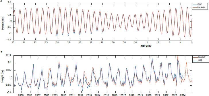
The MSL rise rate of 1.85 mm/yr, obtained from the monthly mean water levels, is much smaller than the 3.1 mm/yr reported by Efraime et al. (2024), who analyzed a time series from the Salvador IBGE station between October 2004 and December 2022. Their rate considers an approximately null vertical land movement according to the local GNSS station. When we analyze the same time interval in our data, we obtain a rate of 2.07 mm/yr, which is still lower than the rate reported by Efraime et al. (2024). The observed difference apparently lies in the data sets used by the two studies. While our time series was based on UHSLC data, with the IBGE data set as auxiliary, Efraime et al. (2025) used the complete IBGE time series. Figure 15a shows the difference between the raw UHSLC and IBGE series for a representative short time interval in 2010. An elevation mismatch between the two series is observed between October 23 and November 3, similar to mismatches detected in other periods. Notable differences also occur in the computations of the monthly-mean sea levels, especially between 2008 and 2015 (Figure 15b).

Figure 15
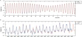
A) A comparison of the IBGE and UHSLC water level time series, showing a period of mismatches between October 23 and November 3, 2010. B) Monthly-mean MSL computed from the IBGE and UHSLC time series between 2004 and 2024.

CONCLUSION

The tides have the largest effect on sea level variability at the entrance of the BTS, with subtidal oscillations explaining less than 2% of the monthly or yearly sea level variance. The mean tidal range is 1.67 m, but ranges can vary six-fold between the smallest and largest values within the tidal nodal cycle. The difference between the maximum and minimum recorded water levels, or the maximum amplitude of intertidal levels, was 3.18 m, about 10% larger than the largest tidal range.

The mean sea level increased at a linear rate of 2.15 mm per year between 2004 and 2024, albeit with significant interannual fluctuations associated with wind speed: consecutive years with a trend of increasing (decreasing) negative wind speeds were associated with a negative (positive) trend in MSL. In addition to a long-term rise in sea level, a trend of increasing frequency and amplitude of long-period waves was detected. However, rising MSL had no apparent impact on the amplitude or phase of the main diurnal and semidiurnal tidal harmonic constituents.

The flooding of the Salvador coastal area inside the bay, associated with extreme water levels, is largely restricted to a filled mangrove area in Baía da Ribeira. Inundation events occur every year, but significant ones take place less often, in association with the 4.4-year tidal cycle. Rising sea level and increasing frequency of subtidal waves have caused an amplification of inundation events. The number of hours with sea level above the inundation threshold increased three-fold between 2022 and 2024. Inundation events are likely more severe in the innermost part of the bay.

DATA AVAILABILITY STATEMENT

the raw data analyzed are available at the University of Hawaii Sea Level Center (UHSLC, station number 334, accessed through the link https://uhslc.soest.hawaii.edu/data/) and at the Brazilian Permanent Geodetic Tide Gauge Network (https://www.ibge.gov.br/geociencias/informacoes-sobre-posicionamento-geodesico/rede-geodesica/10842-rmpg-rede-maregrafica-permanente-para-geodesia.html?=&t=observacao-do-nivel-do-marrmpg).

SUPPLEMENTARY MATERIAL

No supplementary material is available.

ACKNOWLEDGMENTS

C.E.P.T. thanks the Conselho Nacional de Desenvolvimento Cientifico e Tecnológico (CNPQ).

REFERENCES

• Caldwell, P. C., Merrifield, M. A. & Thompson, P. R. 2001. Sea level measured by tide gauges from global oceans as part of the Joint Archive for Sea Level (JASL) since 1846. Bethesda, National Centers for Environmental Information. DOI: https://doi.org/10.7289/v5v40s7W
  » https://doi.org/10.7289/v5v40s7W
• Chen, W.-B. 2025. Gradual strengthening of global oceanic surface winds: Correlations with sea surface temperature and implications for wind power extraction. Heliyon, 11(4), e42788. DOI: https://doi.org/10.1016/j.heliyon.2025.e42788
  » https://doi.org/10.1016/j.heliyon.2025.e42788
• Church, J. A. & White, N. J. 2011. Sea-Level rise from the late 19th to the early 21st century. Surveys in Geophysics, 32(4-5), 585-602. DOI: https://doi.org/10.1007/s10712-011-9119-1
  » https://doi.org/10.1007/s10712-011-9119-1
• Cirano, M. & Lessa, G. C. 2007. Oceanographic characteristics of Baía de Todos os Santos, Brazil. Brazilian Journal of Geophysics, 25(4), 363-387. DOI: https://doi.org/10.1590/s0102-261x2007000400002
  » https://doi.org/10.1590/s0102-261x2007000400002
• Codiga, D. L. 2011. Unified tidal analysis and prediction using the UTIDE Matlab functions. Kingston, University of Rhode Island. DOI: https://doi.org/10.13140/rg.2.1.3761.2008
  » https://doi.org/10.13140/rg.2.1.3761.2008
• De Cai Conrado, E. T., Rocha, R. P., Reboita, M. S. & Cardoso, A. A. 2024. Cyclone classification over the south Atlantic Ocean in centenary reanalysis. Atmosphere, 15(12), 1533. DOI: https://doi.org/10.3390/atmos15121533
  » https://doi.org/10.3390/atmos15121533
• Dodet, G., Melet, A., Ardhuin, F., Bertin, X., Idier, D. & Almar, R. 2019. The contribution of wind-generated waves to coastal sea-level changes. Surveys in Geophysics , 40(6), 1563-1601. DOI: https://doi.org/10.1007/s10712-019-09557-5
  » https://doi.org/10.1007/s10712-019-09557-5
• Egbert, G. D. & Erofeeva, S. Y. 2002. Efficient inverse modeling of barotropic ocean tides. Journal of Atmospheric and Oceanic Technology, 19(2), 183-204. doi: 10.1175/1520-0426(2002)019
  » https://doi.org/10.1175/1520-0426(2002)019
• Efraime, D., Harari, J., de Camargo, R., Soares, S., Mascagni, M.L. & Fetter Filho, A.F.H. 2025. Sea level variation along the Brazilian coastline from the perspective of climate change. Regional Studies in Marine Science, 89, 104309. DOI: https://doi.org/10.1016/j.rsma.2025.104309
  » https://doi.org/10.1016/j.rsma.2025.104309
• Emery, W. J. & Thomson, R. E. 2004. Data analysis methods in physical oceanography. Amsterdam, Pergamon Press. DOI: https://doi.org/10.1016/C2010-0-66362-0
  » https://doi.org/10.1016/C2010-0-66362-0
• Ezer, T. 2013. Sea level rise, spatially uneven and temporally unsteady: why the U.S. East Coast, the global tide gauge record, and the global altimeter data show different trends. Geophysical Research Letters, 40(20), 5439-5444. DOI: https://doi.org/10.1002/2013gl057952
  » https://doi.org/10.1002/2013gl057952
• Franklin, T. S., Lessa, G. C. 2011. O impacto de aterramentos sobre a hidrodinâmica da Baía da Ribeira - Salvador-BA uma investigação atrav´es de modelagem numérica. Revista Brasileira de Geofísica, 29(3): 555-570.
• Franklin, T. S., Lessa, G. C., Teixeira, C. E. P., Santos, F. M., Marta-Almeida, M. & Mendes-Lopes, R. 2026. High-resolution simulations of coastal dispersion of Tubastraea Spp. Larvae from a Large Estuary in Northeast Brazil. SSRN Electronic Coral Reefs. DOI: https://doi.org/10.1007/s00338-026-02817-y
  » https://doi.org/10.1007/s00338-026-02817-y
• Freitas, P. P., Paiva, A. M., Cirano, M.,Mill, G. N.,Costa, V. S., Gabioux M. & França, B. R. L. 2021. Coastal trapped waves propagation along the southwestern Atlantic continental shelf. Continental Shelf Research, 226, 104496. DOI: https://doi.org/10.1016/j.csr.2021.104496
  » https://doi.org/10.1016/j.csr.2021.104496
• Friedrichs, C. T. & Aubrey, D. G. 1988. Non-linear tidal distortion in shallow well-mixed estuaries: a synthesis. Estuarine Coastal and Shelf Science, 27(5), 521-545. DOI: https://doi.org/10.1016/0272-7714(88)90082-0
  » https://doi.org/10.1016/0272-7714(88)90082-0
• Gao, L., Du, H., Huang, H., Zhang, L. & Zhang, P. 2023. Modelling the compound floods upon combined rainfall and storm surge events in a low-lying coastal city. Journal of Hydrology, 627, 130476. DOI: https://doi.org/10.1016/j.jhydrol.2023.130476
  » https://doi.org/10.1016/j.jhydrol.2023.130476
• Genz, F. & Lessa, G. 2015. Twenty-six years of uneven changes in low flows due to different uses and operation of a large dam in a semiarid river. Revista Brasileira De Recursos Hídricos, 20(2), 523-532. DOI: https://doi.org/10.21168/rbrh.v20n2.p523-532
  » https://doi.org/10.21168/rbrh.v20n2.p523-532
• Gramcianinov, C. B., Camargo, R., Campos, R. M., Soares, C. G. & Dias, P. L. S. 2022. Impact of extratropical cyclone intensity and speed on the extreme wave trends in the Atlantic Ocean. Climate Dynamics, 60(5-6), 1447-1466. DOI: https://doi.org/10.1007/s00382-022-06390-2
  » https://doi.org/10.1007/s00382-022-06390-2
• Gramcianinov, C. B., Staneva, J., Camargo, R. & Dias, P. L. S. 2023. Changes in extreme wave events in the southwestern south Atlantic Ocean. Ocean Dynamics, 73(11), 663-678. DOI: https://doi.org/10.1007/s10236-023-01575-7
  » https://doi.org/10.1007/s10236-023-01575-7
• Hamlington, B. D., Bellas-Manley, A., Willis, J. K., Fournier, S., Vinogradova, N., Nerem, R. S., Piecuch, C. G., Thompson, P. R. & Kopp, R. 2024. The rate of global sea level rise doubled during the past three decades. Communications Earth & Environment, 5(1). DOI: https://doi.org/10.1038/s43247-024-01761-5
  » https://doi.org/10.1038/s43247-024-01761-5
• Hamlington, B. D., Cheon, S. H., Piecuch, C. G., Karnauskas, K. B., Thompson, P. R., Kim, K., Reager, J. T., Landerer, F. W. & Frederikse, T. 2019. The dominant global modes of recent internal sea level variability. Journal of Geophysical Research Oceans, 124(4), 2750-2768. DOI: https://doi.org/10.1029/2018jc014635
  » https://doi.org/10.1029/2018jc014635
• Harrison, C. G. A. 2002. Power spectrum of sea level change over fifteen decades of frequency. Geochemistry Geophysics Geosystems, 3(8), 1-17. DOI: https://doi.org/10.1029/2002gc000300
  » https://doi.org/10.1029/2002gc000300
• Hinton, A. C. 1995. Holocene tides of The Wash, U.K.: the influence of water-depth and coastline-shape changes on the record of sea-level change. Marine Geology, 124(1-4), 87-111. DOI: https://doi.org/10.1016/0025-3227(95)00034-v
  » https://doi.org/10.1016/0025-3227(95)00034-v
• IBGE. (2022). Censo 2022: censo cidades. Available from: Available from: https://cidades.ibge.gov.br/brasil/ba/salvador/pesquisa/10101/96387 Access date: 2026 May 28.
  » https://cidades.ibge.gov.br/brasil/ba/salvador/pesquisa/10101/96387
• Jevrejeva, S., Grinsted, A. & Moore, J. C. 2009. Anthropogenic forcing dominates sea level rise since 1850. Geophysical Research Letters , 36(20). DOI: https://doi.org/10.1029/2009gl040216
  » https://doi.org/10.1029/2009gl040216
• Lima, G. M. P. & Lessa, G. C. 2001. The fresh-water discharge in Todos os Santos Bay (BA) an its significance to the general water circulation. Pesquisas em Geociências, 28(2), 85. DOI: https://doi.org/10.22456/1807-9806.20271
  » https://doi.org/10.22456/1807-9806.20271
• Llovel, W., Balem, K., Tajouri, S. & Hochet, A. 2023. Cause of substantial global mean sea level rise over 2014-2016. Geophysical Research Letters , 50(19). DOI: https://doi.org/10.1029/2023gl104709
  » https://doi.org/10.1029/2023gl104709
• Lyddon, C., Brown, J. M., Leonardi, N. & Plater, A. J. 2018. Uncertainty in estuarine extreme water level predictions due to surge-tide interaction. PLoS ONE, 13(10), e0206200. DOI: https://doi.org/10.1371/journal.pone.0206200
  » https://doi.org/10.1371/journal.pone.0206200
• Melo Filho. 2017. Maré meteorológica na costa brasileira (Full Professor Thesis). Federal University of Rio Grande. Available from: Available from: https://sistemas.furg.br/sistemas/sab/arquivos/conteudo_digital/000008808.pdf Access date: 2026 May 28.
  » https://sistemas.furg.br/sistemas/sab/arquivos/conteudo_digital/000008808.pdf
• Muis, S., Aerts, J. C. J. H., Antolínez, J. A. A., Dullaart, J. C., Duong, T. M., Erikson, L., Haarsma, R. J., Apecechea, M. I., Mengel, M., Bars, D. L., O’Neill, A., Ranasinghe, R., Roberts, M. J., Verlaan, M., Ward, P. J. & Yan, K. 2023. Global projections of storm surges using High‐Resolution CMIP6 climate models. Earth’s Future, 11(9). DOI: https://doi.org/10.1029/2023ef003479
  » https://doi.org/10.1029/2023ef003479
• Nicolodi, J. L. & Petermann, R. M. 2010. Mudanças Climáticas e a Vulnerabilidade da zona costeira do Brasil: aspectos ambientais, sociais e tecnológicos. Revista de Gestão Costeira Integrada, 10(2), 151-177. DOI: https://doi.org/10.5894/rgci206
  » https://doi.org/10.5894/rgci206
• Pawlowicz, R., Beardsley, B. & Lentz, S. 2002. Classical tidal harmonic analysis including error estimates in MATLAB using T_TIDE. Computers & Geosciences, 28(8), 929-937. DOI: https://doi.org/10.1016/s0098-3004(02)00013-4
  » https://doi.org/10.1016/s0098-3004(02)00013-4
• Peng, D., Hill, E. M., Meltzner, A. J. & Switzer, A. D. 2019. Tide gauge records show that the 18.61‐year nodal tidal cycle can change high water levels by up to 30 cm. Journal of Geophysical Research Oceans , 124(1), 736-749. DOI: https://doi.org/10.1029/2018jc014695
  » https://doi.org/10.1029/2018jc014695
• Pereira, J., Santos, J. V. B., Lessa, G. C. & Barreto, B. A. The wave climate and well events from ten-year in situ time series at the continental shelf of northern Bahia, Brazil. Ocean and Coastal Oceanography (under review).
• Pickering, M. D., Wells, N. C., Horsburgh, K. J. & Green, J. A. M. 2012. The impact of future sea-level rise on the European shelf tides. Continental Shelf Research , 35, 1-15. DOI: https://doi.org/10.1016/j.csr.2011.11.011
  » https://doi.org/10.1016/j.csr.2011.11.011
• Piecuch, C. G. & Ponte, R. M. 2015. Inverted barometer contributions to recent sea level changes along the northeast coast of North America. Geophysical Research Letters , 42(14), 5918-5925. DOI: https://doi.org/10.1002/2015gl064580
  » https://doi.org/10.1002/2015gl064580
• Ray, R. D. & Merrifield, M. A. 2019. The semiannual and 4.4‐Year modulations of extreme high tides. Journal of Geophysical Research Oceans , 124(8), 5907-5922. DOI: https://doi.org/10.1029/2019jc015061
  » https://doi.org/10.1029/2019jc015061
• Santos, F. M., Lessa, G. C., Cirano, M., Domingues, R. M. & Lentini, C. A. D. 2015. Localized coastal upwelling at the Brazil Current formation zone (13°S). In: XVII Simpósio Brasileiro de Sensoriamento Remoto.
• Schettini, C. A. F., Truccolo, E. C., Mattos, J. A. D. & Benevides, D. C. D. A. 2019. Tides and sea level variability decomposition in the Port of Santos waterway. Brazilian Journal of Oceanography, 67. DOI: 10.1590/s1679-87592019026506707
  » https://doi.org/10.1590/s1679-87592019026506707
• SEFAZ. 2017. Nuvem de pontos LiDAR, carta Salvador, SD-24-X. Available from: Available from: https://cartografia.salvador.ba.gov.br/dados-geoespaciais/baixar-dados-geoespaciais Access date: 2026 Apr. 4.
  » https://cartografia.salvador.ba.gov.br/dados-geoespaciais/baixar-dados-geoespaciais
• Shaw, J., Amos, C. L., Greenberg, D. A., O’Reilly, C. T., Parrott, D. R. & Patton, E. 2010. Catastrophic tidal expansion in the Bay of Fundy, Canada Earth Sciences Sector (ESS) Contribution 20090423. Canadian Journal of Earth Sciences, 47(8), 1079-1091. DOI: https://doi.org/10.1139/e10-046
  » https://doi.org/10.1139/e10-046
• Spicer, P., Huguenard, K., Ross, L. & Rickard, L. N. 2019. High‐frequency tide‐surge‐river interaction in estuaries: causes and implications for coastal flooding. Journal of Geophysical Research Oceans , 124(12), 9517-9530. DOI: https://doi.org/10.1029/2019jc015466
  » https://doi.org/10.1029/2019jc015466
• Sweet, W. V., & Park, J. 2014. From the extreme to the mean: Acceleration and tipping points of coastal inundation from sea level rise. Earth’s Future , 2,579-600. DOI: https://doi.org/10.1002/2014EF000272
  » https://doi.org/10.1002/2014EF000272
• Thévenin, P. J., Pereira, J. & Lessa, G. C. 2019. Shelf-break upwelling on a very narrow continental shelf adjacent to a western boundary current formation zone. Journal of Marine Systems, 194, 52-65. DOI: https://doi.org/10.1016/j.jmarsys.2019.02.008
  » https://doi.org/10.1016/j.jmarsys.2019.02.008
• Truccolo, E. C., Franco, D. & Schettini, C. A. F. 2006. The low frequency sea level oscillations in the northern coast of Santa Catarina, Brazil. Journal of Coastal Research, 39, 547-552. Available at: https://www.researchgate.net/publication/272742146_The_low_Frequency_Sea_Level_Oscillations_in_the_Northern_Coast_of_Santa_Catarina_Brazil
  » https://www.researchgate.net/publication/272742146_The_low_Frequency_Sea_Level_Oscillations_in_the_Northern_Coast_of_Santa_Catarina_Brazil
• Vianna, H. D., Calliari, L. J. & Vianna, S. D. 2020. Inundação e erosão na costa norte do Rio Grande do Sul - Brasil. Estudo de caso: a maré meteorological de outubro de 2016. Revista Brasileira de Geomorfologia, 21(4). DOI: https://doi.org/10.20502/rbg.v21i4.1749
  » https://doi.org/10.20502/rbg.v21i4.1749
• Zheng, C.-W., Li, X.-H., Azorin-Molina, C., Li, C.-Y., Wang, Q., Xiao, Z.-N., Yang, S.-B., Chen, X. & Zhan, C. 2022. Global trends in oceanic wind speed, wind-sea, swell, and mixed wave heights. Applied Energy, 321, 119327. DOI: https://doi.org/10.1016/j.apenergy.2022.119327
  » https://doi.org/10.1016/j.apenergy.2022.119327

• AI USE STATEMENT
  We declare that no generative artificial intelligence (AI) tools were used in the preparation, writing, or editing of this manuscript.
• FUNDING
  This study is a byproduct of the project ‘Assessment and research of sun coral in Todos-os-Santos Bay’, a cooperation agreement between UFBA and PETROBRAS (No 5850.0107361.18.9) regulated by R,D&I investment clauses of the Brazilian Agency of Petroleum, Natural Gas and Biofuels (ANP Resolution 03/2015).

Edited by

• Associate Editor:
  Mauro Cirano

Publication Dates

• Publication in this collection
  07 Sept 2026
• Date of issue
  2026

History

• Received
  17 Dec 2025
• Accepted
  20 May 2026